Project 3: Bayesian Inference

The Objective

In baseball, “launch speed” refers to the speed (in mph) at which the baseball travels after the hitter hits it. Baseball superstar Aaron Judge tends to hit the ball hard. Like, 100 mph launch speed hard.

On June 3, 2023, Judge injured his right big toe crashing into the fence at Dodger Stadium and did not play again for almost two months. The objective of this project is to determine whether the injury and his subsequent recovery affected his launch speed and, if so, quantify how much of a difference there was between pre-injury and post-injury Judge.

The Data

# use this chunk to load any packages you need to do the analysis
# e.g., ggplot2, janitor, purrr

library(dplyr)
library(readr)
library(ggplot2)

# this code should work if you put this file in your Projects subfolder of Math 337
# you may need to open it inside your Math 337 R project
here::i_am("Baseball.qmd")

# this code should work if you make a folder called Data in your Math 337 folder and put the data in it
judge <- readr::read_csv(here::here("Instruction_Data/judge.csv"))

The data for this project comes from Baseball Savant and was obtained primarily using the baseballr package (Dr. Wynne did a bit of data wrangling with the originally obtained data). It contains launch speed data about the 55 baseballs Aaron Judge hit into play in the month before his injury and the 62 baseballs he hit into play in the month after returning from injury.

Section 1: The Prior Distribution

Goal 1:
I aimed to explore what Aaron Judge’s launch speeds might look like before observing any data by simulating from a prior distribution. I adjusted the parameters so that the simulated speeds remained realistic. For example, rarely exceeding 120 mph, which a baseball expert (Gigi) confirmed is essentially impossible. I used histograms to visualize the results, allowing me to see plausible ranges and verify that the prior expectations were reasonable, thus providing a sensible starting point for the Bayesian analysis.

#general idea of what we want to get
#y1: need mu1 and sigma
  #mu1: t1, sigma, kappa0
    #sigma: alpha0, lambda0
#WLOG y2
#set t1, t1, alpha0, lambda0, kappa0

#set seed
set.seed(1222)
sim_prior_pred <- function(R = 1000,
                           t1 = 99,#expected mean preinjury
                          t2 = 90,#expected mean postinjury
                          kappa0 = 5,# strength of prior
                      alpha0 = 30,#gamma shape 4 precision
                      lambda0 = 1000#gamma rate 4 precision
) {
  #Step 1: Draw precision v from Gamma(alpha0/2, lambda0/2) to then get sigma
  v2 <- rgamma(R, shape = alpha0/2, rate = lambda0/2)
  sigma <- 1 / sqrt(v2)
  
  #Step 2: Draw mu1, mu2 given sigma and kappa0
  mu1 <- rnorm(R, mean = t1, sd = sigma / sqrt(kappa0))
  mu2 <- rnorm(R, mean = t2, sd = sigma / sqrt(kappa0))
  
  #step 3: Draw y1,y2 based on mu1/2 and sigma
  y1 <- rnorm(R, mean = mu1, sd = sigma) #pre-injury
  y2 <- rnorm(R, mean = mu2, sd = sigma) #post-injury
  
  #put it into a list to then make visuals for
  list(sigma = sigma, mu1 = mu1, mu2 = mu2, y1 = y1, y2 = y2)
}

#run it
#putting it into histograms
res <- sim_prior_pred()
hist(res$y1) #pre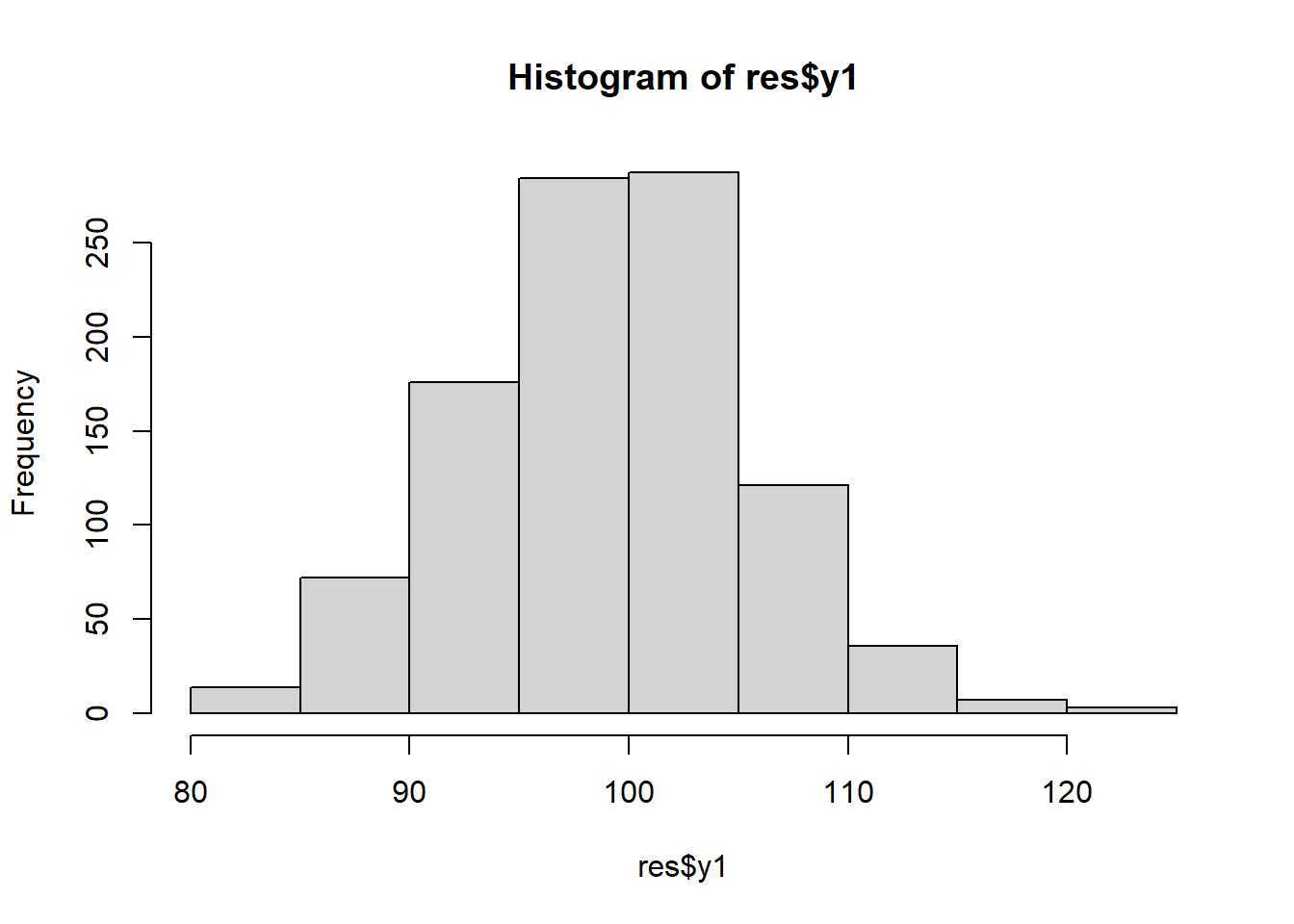

hist(res$y2) #post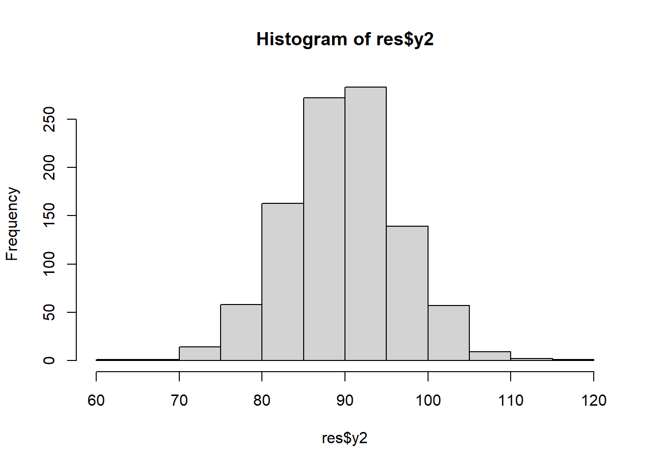

Section 2: The Observed Data

Goal 1:
Based on the numerical and graphical summaries, Aaron Judge’s launch speeds appear slightly lower after the injury, but the change is not dramatic. The average launch speed decreased from 99.3 mph (pre-injury) to 97.9 mph (post-injury). The spread of the data also changed: pre-injury launch speeds had a slightly larger standard deviation (12.3) compared to post-injury (11.0), suggesting that his pre-injury performance was a bit less consistent. The boxplots reflect this, showing a slightly tighter cluster of launch speeds in the post-injury period.

Overall, Judge’s post-injury launch speeds are slightly lower but also more consistent. So based on launch speed alone, he appears to be performing at a similar level pre- and post-injury.

#summarize data from the csv
launch_summary <- judge |>
  select(injury, launch_speed) |> #selecting just these
  group_by(injury) |>
  summarise(
    mean = mean(launch_speed), #look at averages
    median = median(launch_speed), #look at medians
    sd = sd(launch_speed), #get the sd
    min = min(launch_speed), #whats the lowest
    max = max(launch_speed) #whats the highest
  )
launch_summary

# A tibble: 2 × 6
  injury  mean median    sd   min   max
  <chr>  <dbl>  <dbl> <dbl> <dbl> <dbl>
1 Post    98.0   100.  11.0  66.3  116.
2 Pre     99.3   102   12.3  69.7  117.

#started with histograms but liekd the idea of a boxplot instead
#setting the order for visual purposes
  #cause og it was post on the left pre on the right
    #not the biggest of deals but ya know... i cared
judge$injury <- factor(judge$injury, levels = c("Pre", "Post")) #had to look up to get help on how to do this

ggplot(judge, aes(x = injury, y = launch_speed, fill = injury)) +
  geom_boxplot() +
  labs(
    title = "Launch Speed Pre vs Post Injury",
    y = "Launch Speed (mph)"
  ) +
  scale_fill_manual(values = c("pink", "lightblue")) +
  theme_light()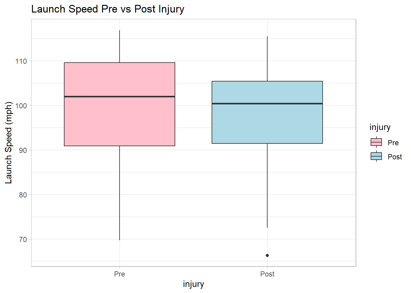 

#ummmm why does he look more consistent afterwards?

Section 3: Creating the Posterior Distribution

Goal 1:
I used Gibbs sampling algorithm to generate posterior distributions for the pre-injury mean (mu1) and post-injury mean (mu 2) and standard deviation (sigma) of Judge’s launch speeds. The overall goal of the Gibbs sampler is to update one parameter at a time using the current values of the others, over and over, so that eventually the sequence of draws settles down and represents the full joint posterior distribution of all the parameters. In other words, by repeatedly sampling in this way, we let the algorithm “learn” the relationships between the parameters and produce realistic combinations of mu1, mu2, and sigma based on both our data and prior beliefs.

# set seef
set.seed(1222)
#parameters from prior predictive function from section 1
t1 <- 99
t2 <- 90
kappa0 <- 5
alpha0 <- 30
lambda0 <- 1000

#splitting data to use:
y1 <- judge$launch_speed[judge$injury == "Pre"]
y2 <- judge$launch_speed[judge$injury == "Post"]
n1 <- length(y1)
n2 <- length(y2)

#storage matrix
param <- matrix(0, nrow = 5000, ncol = 3)

#initial values from data
mu1 <- mean(y1)
mu2 <- mean(y2)
sigma <- sd(c(y1,y2))

#Gibbs Sampelr
#iterating 5000 times
for (i in 1:5000){
  #sample mu1 given mu 2 and sigma
  mu_p1 <- (sum(y1) + kappa0*t1) / (n1 + kappa0)
  sd_p1 <- sigma / sqrt(n1 + kappa0)
  mu1 <- rnorm(1, mean = mu_p1, sd = sd_p1) #updated mu1
  
  #same for mu2 given mu 1 sigma
  mu_p2 <- (sum(y2) + kappa0*t2) / (n2 + kappa0)
  sd_p2 <- sigma / sqrt(n2 + kappa0)
  mu2 <- rnorm(1, mean = mu_p2, sd = sd_p2) #updated mu2
  
  #Sample sigma given mu1 and mu2
  #putting it in parts cauuuuse i caaan
  #precision v = 1/sigma^2
  
  #post shape based off of formula sheet
  alpha_p <- alpha0 + n1 + n2
  
  #doing all this shabam for lambda_p based on formula sheet
  # Compute Sums + prior terms (the kappa segment)
  sum1 <- sum((y1 - mu1)^2)
  sum2 <- sum((y2 - mu2)^2)
  kappa_segment <- kappa0*((mu1 - t1)^2 + (mu2 - t2)^2)
  
  lambda_p <- lambda0 + sum1 + sum2 + kappa_segment
  
  #sample v
  v <- rgamma(1, shape = alpha_p/2, rate = lambda_p/2)
  sigma <- 1/sqrt(v) #precision thing i commented earlier
  
  #store results
  param[i,] <- c(mu1, mu2, sigma)
}

#burn in removal
param_converged <- param[1001:5000,]

#plots for goal 2
#par(mfrow=c(2,2))
plot(param_converged[,1], type="l", main="mu1")

plot(param_converged[,2], type="l", main="mu2")

plot(param_converged[,3], type="l", main="sigma")

Goal 2:
After discarding the first 1,000 burn-in iterations, I plotted the posterior samples for mu1, mu2, and sigma. Each plot shows how the sampled values evolve over the iterations. The plots fluctuate around stable levels without any noticeable trends or drifts, which indicates that the chains have likely converged to their stationary distributions.

Section 4: Interpreting the Posterior Distribution

Goal 1:
The posterior distribution of the difference in launch speeds (mu1 - mu2) is mostly positive, suggesting that pre-injury launch speeds were generally higher than post-injury. A small fraction of draws are negative but overall the updated beliefs indicate a slight decrease in launch speed following the injury.

# get last 4000 draws
mu1_post <- param_converged[,1] #mu1 is pre
mu2_post <- param_converged[,2] #mu 2 is post

# Compute posterior difference
diff_post <- mu1_post - mu2_post

#plot
hist(diff_post,
     breaks = 40,
     col = "lightblue",
     main = "Posterior Distribution of mu1 − mu2",
     xlab = "mu1 − mu2")

#90% credible interval
#taking quantile from diff_post which is the difference of mu1 and mu 2
quantile(diff_post, c(0.05,0.95))

       5%       95% 
-1.288514  5.147772 

Goal 2:
The 90% credible interval for mu1 − mu2 ranges from about -1.3 to 5.1 mph. This suggests that Judge’s pre-injury launch speed was generally slightly higher than post-injury. However, there is some uncertainty, meaning we cannot be completely sure of the exact difference. While a small decrease is most likely, it’s still possible that the launch speed stayed the same. Overall, it is most likely that the injury caused a minor decrease in launch speed, but the effect is small and not dramatic.

Goal 3:
Based on the posterior distribution and the 90% credible interval for mu1 − mu2, Judge’s launch speeds post-injury are very similar to those pre-injury. While there is some indication of a small decrease in launch speed, the effect is minor. Overall, the analysis suggests that Judge returned as essentially the same player in terms of launch speed, with any changes being relatively minor rather than life-changing.

Appendix: Conceptual Details

Bayesian inference is a way of updating your beliefs about something uncertain using both what you already know and the new data you see. Before looking at the data, we start with a prior distribution, which is basically our guess or expectation. For example, I thought Aaron Judge’s average launch speed might be around 99 mph based on my very limited baseball knowledge. The likelihood function tells us how likely the data we actually saw is, given different possible values. Basically, how well different guesses match the real launch speeds. The posterior distribution combines the prior and the data to give an updated guess, showing what values are most likely after seeing the evidence. This way, we can mix what we thought before with what we actually observed to make a more informed conclusion.