Project 2: Hypothesis Tests

The Objective

You are working for a pharmaceutical company that is testing a new treatment for long COVID. You are tasked with analyzing the collected data to determine whether there is sufficient evidence of an effect of treatment on the risk of long COVID in the at-risk population. Before any data is collected, you should investigate the sensitivity of your test to differences in the assumptions about the collected data, e.g., number of patients enrolled, true population proportion of long COVID among treated or untreated adults, etc.

The Data

Show code

library(dplyr)
library(ggplot2)
library(purrr)

Show code

# this code should work if you put this file in your Projects subfolder of Math 337
# you may need to open it inside your Math 337 R project
here::i_am("LongCOVID.qmd")

## the data from Maier, Kowalski-Dobson, et al.
long_covid <- data.frame(
  symptoms = c(rep(1, 23), rep(0, 106), rep(1, 81), rep(0, 214)),
  # symptoms = 1 if symptoms remain after 90 days, 0 if symptoms are gone within 90 days
  vax = c(rep("treatment", 129), rep("control", 295))
  # treatment = vaccinated, control = unvaccinated
)
# table(), xtabs() and tabyl() (from janitor) will all produce tables of this data,
# coercing both symptoms and treatment to factors automatically

The data in long_covid comes from Maier, Kowalski-Dobson, et al. (2024), “Reduction in long-COVID symptoms and symptom severity in vaccinated compared to unvaccinated adults,” and was collected on employees and students at the University of Michigan who tested positive for COVID-19 between October 2020 and December 2022. The specific data here is restricted to pre-Omicron variant COVID-19 (roughly October 2020 - December 2021).

Section 1: Permutation Test for Effect of Vaccination

Goal 1:

Show code

#like in class from estimating alphas
#observing diff in proportions different then in class when we observed difference in means.
perm_test <- function(df, R = 999, alternative = "t") {
#df: data
  #column 1: response (0 = no long covid and 1 = long covid) (symptoms)
  #column 2: group (treatment or control) (vax)
#R: number of perm resamples to generate
  # alternative: type of test (l = left, r = right, t = two-sided)
  
#check the alt argument is valid
  assertthat::assert_that(
    alternative %in% c("l", "r", "t"),
    msg = 'Alternative must be "l", "r", or "t" '
  )
  
#get the response variable (long COVID yes 1/no 0)
  response <- df[, 1, drop = TRUE]
  
#get and convert the group variable to a factor (to separate treatment/control)
  group <- as.factor(df[, 2, drop = TRUE])
  
#storing group names
  control <- levels(group)[1] #control
  treatment <- levels(group)[2] #treatment (cause alphabetical order)
  

#STEP 1: Compute obs diff in proportions
  #mean of 0 and 1 values is sample prop
  #have to get proportions since numbers are binary and not like values
  p1_obs_control <- mean(response[group == control])  # props of long COVID in group1 (control)
  p2_obs_treatment <- mean(response[group == treatment])  # props of long COVID in group2 (treatment)
  
  #observed t.stat: diff in proportions
  diff_obs <- p1_obs_control - p2_obs_treatment
  

#STEP 2: Simulate permutation null dist

  diff_samp_prop <- function(ind, y) {
  # ind: indices assigned to treatment group
  #y: vector containing the response vals
    #mean(y[ind]): simulated treatment group proportion
    #mean(y[-ind]): simulated control group proportion
    
    diff_prop <- mean(y[ind]) -  mean(y[-ind]) #diff in proportions
    
    return(diff_prop)
  }
  
  #under the null hypothesis: group assignment doesnt matter
  #so rand move around who is in g1 vs g2
  index_sim <- replicate(
    R,
    {
      # randomly assign which patients are in the treatment group
      sample(seq_along(response), sum(group == treatment), replace = FALSE)
    }
  )
  
  # --- part 3: compute simulated differences for each permutation ---
  diff_props_sim <- apply(
    index_sim,   # matrix of simulated treatment indices
    2,           # apply function to each column
    diff_samp_prop, # custom helper function
    y = response
  )

#STEP 3: Combine sim and obs stats
  
  diff_all <- c(diff_props_sim, diff_obs)

#STEP 4: Compute permutation pvals
 #left: probability of seeing a value <= obs
  p_left <- mean(diff_all <= diff_obs)
  
  #right: probability of seeing a value >= observed
  p_right <- mean(diff_all >= diff_obs)
  
  #two: smallest tail × 2
  p_two_sided <- min(p_left, p_right) * 2
  
#return results
  invisible(
    list(
      obs_test_stat = diff_obs,   # observed difference in proportions
      all_test_stat = diff_all,   # vector of simulated + observed stats
      p.val = dplyr::case_when(   # pick correct p-value type
        alternative == "l" ~ p_left,
        alternative == "r" ~ p_right,
        alternative == "t" ~ p_two_sided
      )
    )
  )
}
  
#testing:
set.seed(1222)
results <- perm_test(long_covid, R = 999, alternative = "t")

#obs diff and p-value
obs_diff <- results$obs_test_stat   #observed diff
diff_all <- results$all_test_stat
p_val <- results$p.val   #pval

#plot: histogram
hist(
  diff_all,
  main = "Permutation Null Distribution",
  xlab = "Difference in Proportions (p1 - p2)"
)

#observed statistic line
abline(v = obs_diff, col = "red", lwd = 2)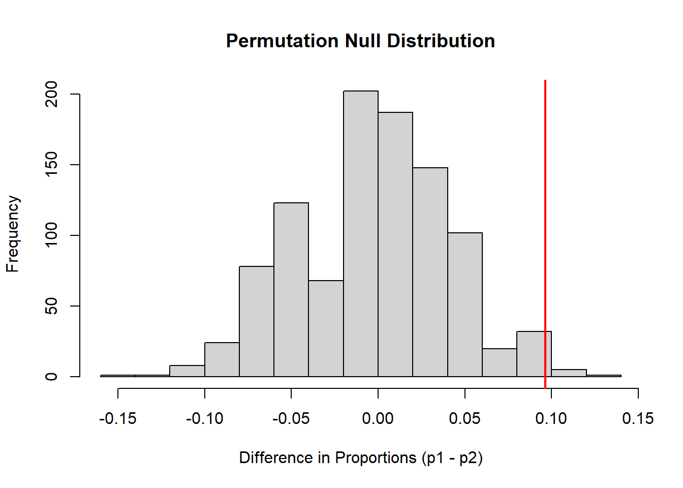

Goal 2:

The observed difference in proportions between the control and treatment groups was 0.096. This means that the treatment group had a 9.6% lower risk of developing long COVID compared to the control group.

The null hypothesis assume that the treatment has no effect on the likelihood of developing long COVID. Comparing the observed difference resulted in a p-value of 0.014. Since this p-value is less than the significance level (0.05), then there is sufficient evidence to reject the null hypothesis. This means that getting treated will reduce the risk of developing long COVID.

Section 2: Analyzing the Company’s New Treatment

Goal 1:

A type I error would mean that the company comes to the conclusion that treatment for long COVID does reduce the risk of long COVID when in reality it does not. The consequence would be a waste of time, money and resources. The company approving and promoting an ineffective treatment would lead to people buying something that wouldn’t work. This not only can impact the credibility of the company but also can stall further medical research from looking further into for (a better/an actual) effective treatment.

A type II error would mean the company comes to the conclusion that the treatment doesn’t work when in reality it does reduce the risk of long COVID. The consequence would be delayed treatment, preventing patients from benefiting.

While both errors are important, depending on the perspective, one might be worse then the other. From the patient point of view, type I error could be more harmful due to the risk of giving false information. From a company point of view, a type II error is more costly, spending more money trying to find a treatment that already exists.

Type I error in this context might be more serious due to the fact that it could impact credibility and has ethical consequences.

Goal 2:

Show code

set.seed(1222)
p_values <- replicate(
  1000, #sim 1000 times
  {
    #null: both groups have same long COVID rate 20%
      #using binom since its 0's and 1's
    group1_response <- rbinom(100, size = 1, prob = 0.20) 
    group2_response <- rbinom(100, size = 1, prob = 0.20)
    
    #combine into df for perm_test
    fake_data <- data.frame(
      response = c(group1_response, group2_response),
      group = c(rep("treatment", 100), rep("control", 100))
    )
    
    #perm test and get pval
    perm_test_sim<- perm_test(fake_data, R = 999, alternative = "t") |>
      purrr::pluck("p.val")
  }
)

#mean(p_values<=0.05) this estimated alpha at just one pt 0.05

# checking multiple alpha levels vvv
alpha_vals <- seq(0.01, 0.10, by = 0.01)

# estimated Type I Error at each alpha using sapply
type1_error <- sapply(alpha_vals, function(a) mean(p_values <= a))

# simple plot
plot(alpha_vals, type1_error,
     xlab = expression(alpha),
     ylab = "Estimated Type I Error Rate",
     main = "Calibration of Permutation Test")
abline(0, 1, col = "magenta")  # ideal line y = x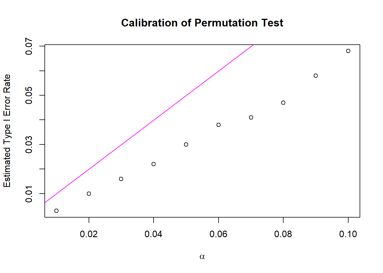

Goal 2:

I first had to simulate the null hypothesis using the binomial distribution. This is because the response variables is binary (1’s and 0’s).

Then evaluated the calibration of the permutation test by estimating type I error rate at multiple significant levels. The result was that the observed type I error is consistently a little below the nominal alpha level. By plotting the ECDF of these p-values against the 1-1 line, visually you can see how the ECDF points lies below the ideal line (magenta). This means the test is less likely to make false positives but may reduce the tests power.

GOAL 3:

Show code

set.seed(1225)
p_values_reduc <- replicate(
  1000, 
  { 
    #generate responses
    group1_response_reduc <- rbinom(100, size = 1, prob = 0.20)  #20% long COVID rate
    group2_response_reduc <- rbinom(100, size = 1, prob = 0.15)  #15% long COVID rate 
              #(25% reducton since 0.20/.75= 0.15)
    
    #combine into df
    fake_data <- data.frame(
      response = c(group1_response_reduc, group2_response_reduc),
      group = c(rep("control", 100), rep("treatment", 100))
    )
    
    # run permutation test and extract p-value
    perm_test_simR <- perm_test(df = fake_data, R = 999, alternative = "t") |>
      purrr::pluck("p.val")
  }
)
alpha <- 0.05
#estimated power
mean(p_values_reduc <= alpha)

[1] 0.118

The control group had a 20% long COVID rate and the treatment group had a 15% rate. I then ran the permutation test where the p-values were recorded.

The proportion of simulations where the test rejected the null (at alpha = 0.05) was 11.8%. This means that the permutation test is unlikely to detect a 25% reduction in risk of long COVID.

Section 3: Sensitivity Analysis

Show code

#parameters I could change
n <- 100
#if changing sample size instead use to give 10 conditions:
#sample_sizes <- seq(20, 200, length.out = 10)
alpha <- 0.05

#changing relative risk
RR <- 1  # fixed at 1 for now

#control probabilities
p_control_vals <- seq(0.10, 0.25, length.out = 10)
#prob_control <- 0.20 if changing treatment

#treatment probabilities
#p_treatment_vals <- seq(0.10, 0.25, length.out = 10) if changing treatment
p_treatment <- 0.20  #fixed otherwise

fisher_test <- function(p_control) { #change to p_treat if changing treatment
  p_values <- replicate(
    1000,
    {
      group_treat <- rbinom(n, 1, p_treatment)
      group_ctrl  <- rbinom(n, 1, p_control)
      
      tbl <- table(
        response = c(group_treat, group_ctrl),
        group    = c(rep("treatment", n), rep("control", n))
      )
      fisher.test(tbl)$p.value
    }
  )
  #estimated power
  mean(p_values <= alpha)
}

#apply the function to all treatment probabilities
  #change "p_control_vals to p_treatment if changing that
power_estimates <- sapply(p_control_vals, fisher_test)
  #sapply applies my function to the vectors and outputs a vector (??) of numbers

# Plot with help of chat to understand what the heck im looking at
plot(p_control_vals, power_estimates, type = "b", pch = 16, col = "magenta",
     xlab = "Control probability of Long COVID",
     ylab = "Estimated power",
     main = "Sensitivity Analysis: Power vs Control Probability")
abline(h = alpha, col = "grey", lty = 2)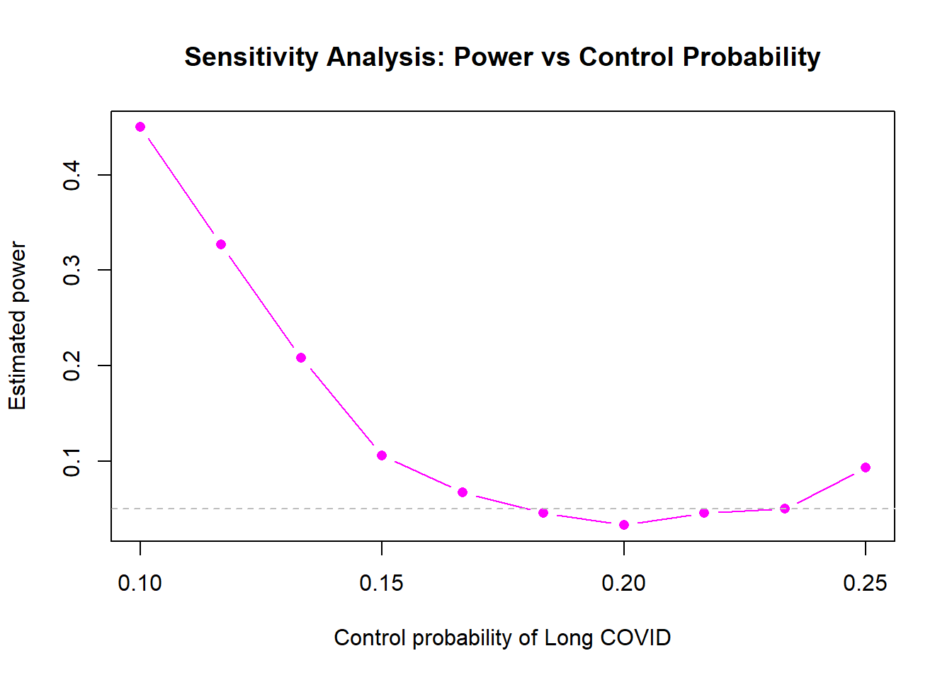

I performed the sensitivity analysis on varying control group probability to see if it affects the power of the test. I picked 10 control probabilities between 0.10 and 0.25 with the treatment probability fixed at 0.20.

The results showed that when the control probabilty is greater or less than 0.20, the estimated power is high (highest at probability 0.10). Meaning it detects the difference between the treatment and control groups more frequently when the control probability isnt 0.20. When the control group probability equal to the control probabilty estimated power was at its lowest.

However, even in these conditions, the estimated power stays low and never reached that common 80% threshold. This may indicate that some other change needs to be made like a larger sample size or bigger differences between control and treatment probabilities.