Modeling Encelia Species Project

Packages Used In This Analysis

library(here)
library(readr)
library(ggplot2)
library(dplyr)
library(rsample)
library(purrr)
library(yardstick)
library(tidyr)
library(gt)
library(broom)

Motivation and Context

The Iris dataset is a small dataset from 1936 that includes three species of Iris: Iris setosa, Iris virginica, and Iris versicolor. Over time, the dataset’s association with eugenics has led to controversy. As a result, several alternative datasets have been developed to replace it, including the Palmer Penguin dataset.

In class, we created a similar dataset featuring flowers found in the Fullerton Arboretum: Encelia californcia and Encelia farinosa. Both species are native to California. Encelia californica typically grows in coastal environments, while Encelia farinosa is known for its resilience in drier areas.

Main Objective

The goal of this project was to develop a predictive model that can accurately classify two types of Encelia flowers based on their physical traits. By analyzing measurements ( number of rays, disk diameter, ray diameter, and stem length) the aim was to determine whether these features can reliably distinguish the two species. Ultimately, this type of model could help automate identification and improve our understanding of the differences between these flower types.

Design and Data Collection

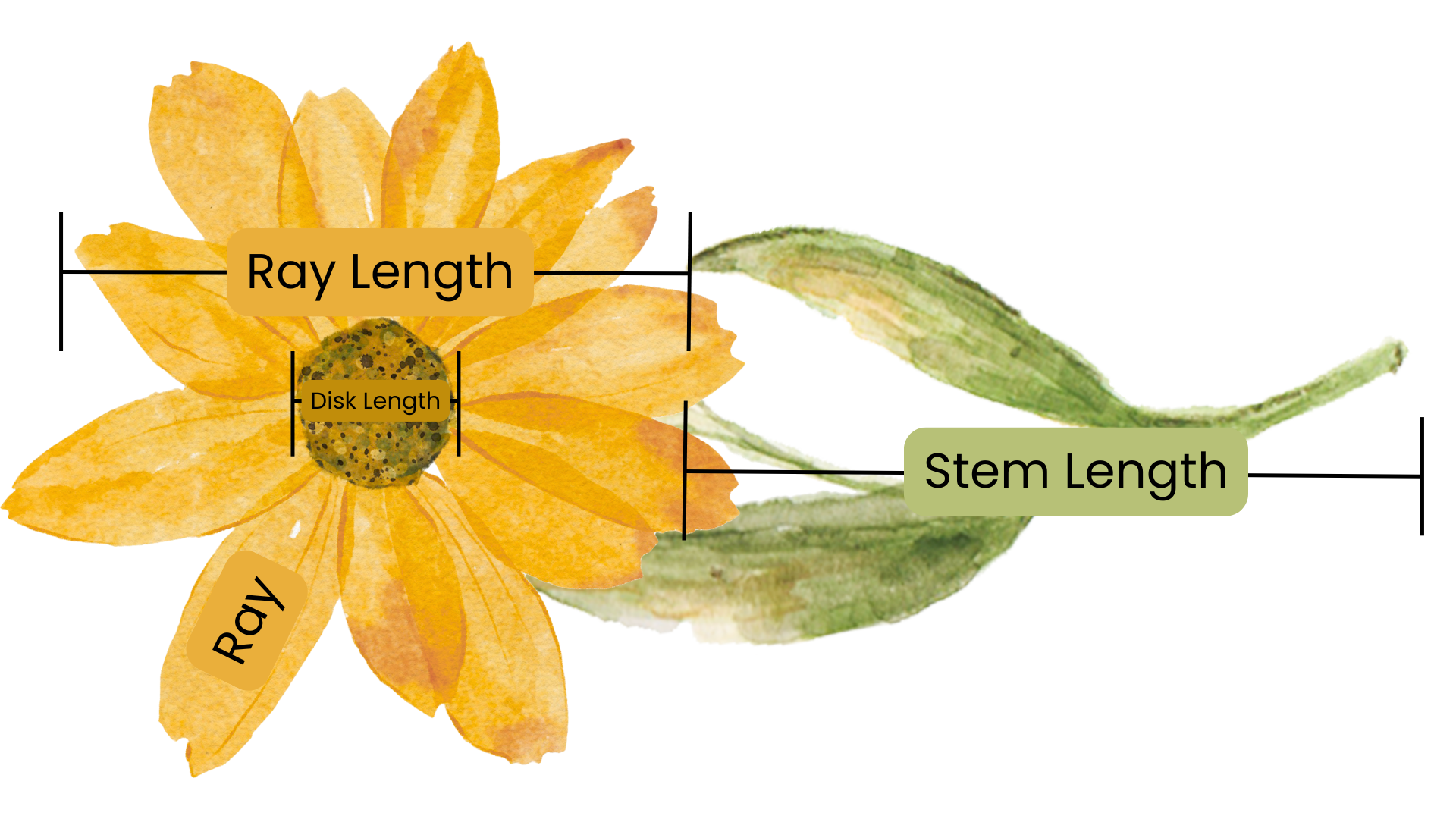
As a class, we went to the Fullerton Arboretum and recorded data on Encelia californica and Encelia farinosa. We split into pairs and collected 10 data samples for each species. The features we measured included the number of rays, the diameter of the disk (in inches), the ray diameter (in inches), and the stem length (in inches). There is some missing data for stem length because one pair of classmates measured a different feature instead. While this isn’t a major issue, it’s worth noting.

Another point about stem length: these flowers tend to have very long stems. My partner and I measured stem length from the bud to the nearest branch-off point. I’m fairly certain most of the class used the same approach, but I can’t say for sure. Overall, all measurements were collected by hand using a ruler, so they are approximate rather than precise.

Training-Test Split

The dataset was fairly clean (which is ideal for recreating something like the Iris dataset) so no major data cleaning was needed. I only made a small change by converting the Species values from “C” and “F” to “Californica” and “Farinosa” for clarity. I also turned the Species column into a factor so we could use it in the models.

encelia <- read_csv("ProjectData/encelia_class.csv") |>
  mutate(
    Species = if_else(Species == "C", "Californica", "Farinosa"),
    Species = as.factor(Species)
  )

I then split the Encelia data into a training set and a test set, with 80% of each species included in the training set and the remaining 20% in the test set. The training set will be used to fit the model, while the test set will be used to evaluate how well the model performs on unseen data.

set.seed(3)
encelia_split <- initial_split(
  encelia,
  strata = Species,
  prop = .8 #training set is 80% of each species
)
encelia_train <- training(encelia_split)
encelia_test <- testing(encelia_split)

Exploratory Data Analysis

The dataset is fairly straightforward. Using ggplot, I created jitter plots to visually examine the differences in variables between the species. I also made a table summarizing the numeric values to provide more precise averages for each flower species’ characteristics. The most noticeable difference is that Encelia californica has longer stems than Encelia farinosa. Encelia californica also has more rays and is overall slightly larger than Encelia farinosa.

Knowing these small measurement differences between species is important. For example, if you pick up a flower at random, understanding the characteristics of each species can help you identify which one you have. Models essentially do the same thing in which they use measurable traits to predict species and assist with classification.

labels <- c(
  number_rays = "Number of Rays",
  disk_diameter = "Disk Diameter (in)",
  ray_diameter = "Ray Diameter (in)",
  stem_length = "Stem Length (in)"
)
encelia_long <- encelia_train |>
  pivot_longer(cols = c(number_rays, disk_diameter, ray_diameter, stem_length),
               names_to = "Trait",
               values_to = "Value")

ggplot(encelia_long, aes(x = Value, y = Species)) +
  geom_jitter(height = 0.1, alpha = 0.8, color = "#F17300") +
 facet_wrap(~ Trait, scales = "free_x", 
             labeller = labeller(Trait = labels)) +
  labs(title = "Trait Distributions by Species",
       y = "Species") +
  theme(strip.text = element_text(face = "bold"),             
    axis.title = element_text(size = 18),        
    axis.text = element_text(size = 14),         
    plot.title = element_text(size = 16, face = "bold")) +
  theme_light()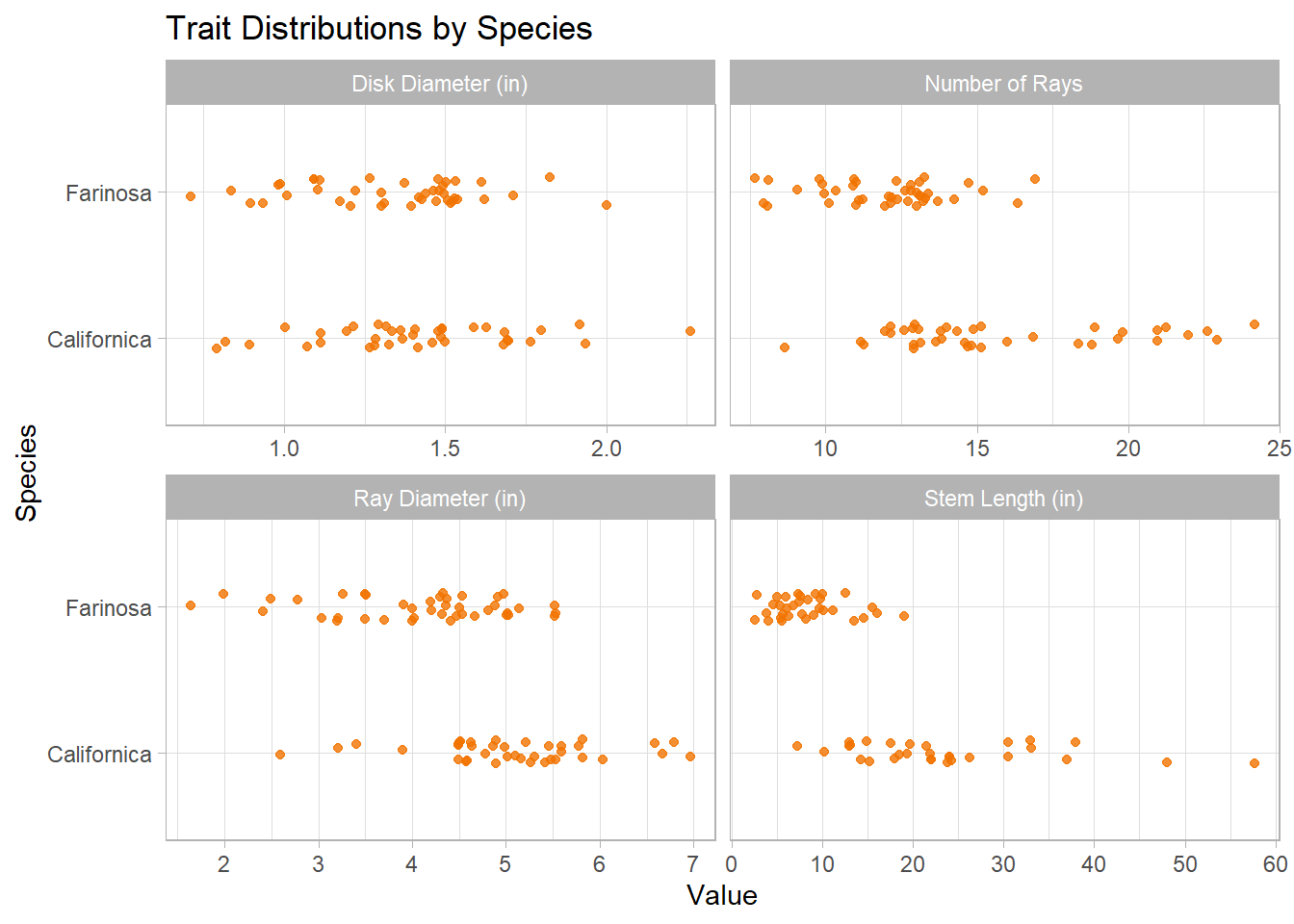

summary_table <- encelia_train |>
  group_by(Species) |>
   summarize(mean.ray = round(mean(number_rays, na.rm = TRUE), digits = 2),
            mean.disk = round(mean(disk_diameter, na.rm = TRUE), digits = 2),
            mean.rayd = round(mean(ray_diameter, na.rm = TRUE), digits = 2),
            mean.stem = round(mean(stem_length, na.rm = TRUE), digits = 2),
            .groups = "drop")
summary_table |>
  pivot_longer(-Species, names_to = "Variable", values_to = "Value") |>
  mutate(Variable = recode(Variable,
                        "mean.ray" = "Number of Rays (mean)",
                        "mean.disk" = "Disk Diameter (mean)",
                        "mean.rayd" = "Ray Diameter (mean)",
                        "mean.stem" = "Stem Length (mean)",)) |>
  pivot_wider(names_from = Species, values_from = Value) |>
  gt() |>
  tab_header(title = "Trait Summary by Species") |>
  cols_align(align = "left") |>
  opt_stylize(style = 6, color = "green") |>
  tab_options(
    table.font.size = px(16),
    heading.title.font.size = px(20),
    heading.subtitle.font.size = px(14),
    data_row.padding = px(3),
    table.width = pct(100)
  )

Trait Summary by Species
Variable	Californica	Farinosa
Number of Rays (mean)	15.84	11.93
Disk Diameter (mean)	1.42	1.33
Ray Diameter (mean)	5.08	4.09
Stem Length (mean)	23.70	8.37

Modeling

What is logistic regression?

Logistic regression is a statistical modeling technique used to predict the probability of an event occurring. In our case, it predicts the probability that a flower belongs to a particular species. Logistic regression uses the logistic function to ensure predictions fall between 0 and 1, representing the likelihood of the flower being classified as one species or the other.

Why are you doing logistic regression?

I’m using logistic regression to classify the species of the Encelia flower based on their measured traits, like number of rays, disk diameter, ray diameter, and stem length. Since there are just two species (Californica vs. Farinosa), logistic regression helps me model how these traits relate to the chance that a flower belongs to one species or the other. This way, I can figure out which traits matter most for telling them apart and predict the species of new flowers based on their measurements.

encelia_prediction <- function(split){
  train <- analysis(split)
  valid <- assessment(split)
  
  glm_all <- glm(Species ~ number_rays + disk_diameter + ray_diameter + stem_length, data = train, family = "binomial")
  glm_stemray <- glm(Species ~ stem_length + ray_diameter, data = train, family = "binomial")
  glm_null <- glm(Species ~ 1, data = train, family = "binomial")
  valid_predictions <- valid |>
    mutate(
      pred_all = predict(glm_all, newdata = valid, type = "response"),
      pred_stemray = predict(glm_stemray, newdata = valid, type = "response"),
      pred_null = predict(glm_null, newdata = valid, type = "response")
    )
  return(valid_predictions)
}

Why did you choose each model that you are considering?

I picked three models to see how well different traits can predict the species.

All traits model (pred_all): This one uses all the traits we measured (rays, disk diameter, ray diameter, and stem length) to see how well the full set works for telling the species apart.

Rays and stem length model (pred_stemray): I chose just rays and stem length because those showed the biggest differences between the species in the data. This simpler model checks if these two key traits alone can still make good predictions.

Null model (pred_null): This one doesn’t use any traits at all. It just guesses based on how common each species is. It’s a baseline to compare the other models against.

By comparing these, I can figure out which traits really matter and if the simpler model does almost as well as the full one.

Why are you using cross-validation? How does it work?

I’m using cross-validation to see how well my models will work on new data they haven’t seen before. Instead of just testing on the same data the model was trained on, cross-validation splits the data into chunks (called folds) and tests the model on each chunk while training it on the rest.

set.seed(1)
encelia_cv <- vfold_cv(
  encelia_train, 
  v = 4
  )

mapped_predictions <- map(
  encelia_cv$splits,
  encelia_prediction
)
mapped_predictions_df <- mapped_predictions|>
  bind_rows(
    .id = "fold"
  )
mapped_predictions_df|>
  select(Species, fold, pred_all, pred_stemray, pred_null)

# A tibble: 79 × 5
   Species     fold   pred_all pred_stemray pred_null
   <fct>       <chr>     <dbl>        <dbl>     <dbl>
 1 Californica 1      2.22e-16      0.0317      0.458
 2 Californica 1      2.22e-16      0.0720      0.458
 3 Californica 1      2.22e-16      0.0185      0.458
 4 Californica 1      2.22e-16      0.00106     0.458
 5 Californica 1     NA            NA           0.458
 6 Californica 1      2.22e-16      0.0354      0.458
 7 Farinosa    1      1   e+ 0      0.986       0.458
 8 Farinosa    1      2.22e-16      0.286       0.458
 9 Farinosa    1      2.22e-16      0.920       0.458
10 Farinosa    1      1   e+ 0      0.955       0.458
# ℹ 69 more rows

pred_all <- mapped_predictions_df |>
  pivot_longer(
    cols = starts_with("pred"),
    names_to = "model",
    values_to = ".pred_Farinosa"
  ) |>
  mutate(
    .pred_Californica = 1 - .pred_Farinosa
  )

pred_all |>
  select(Species, model, fold, .pred_Californica, .pred_Farinosa)

# A tibble: 237 × 5
   Species     model        fold  .pred_Californica .pred_Farinosa
   <fct>       <chr>        <chr>             <dbl>          <dbl>
 1 Californica pred_all     1                 1           2.22e-16
 2 Californica pred_stemray 1                 0.968       3.17e- 2
 3 Californica pred_null    1                 0.542       4.58e- 1
 4 Californica pred_all     1                 1           2.22e-16
 5 Californica pred_stemray 1                 0.928       7.20e- 2
 6 Californica pred_null    1                 0.542       4.58e- 1
 7 Californica pred_all     1                 1           2.22e-16
 8 Californica pred_stemray 1                 0.981       1.85e- 2
 9 Californica pred_null    1                 0.542       4.58e- 1
10 Californica pred_all     1                 1           2.22e-16
# ℹ 227 more rows

brier_all_models <- pred_all |>
  group_by(model, fold) |>
  brier_class(
    truth = Species,
    .pred_Californica
  )
brier_summary <- brier_all_models |>
  ungroup() |>
  group_by(model) |>
  summarize(
    mean_brier = mean(.estimate),     
    se_brier = sd(.estimate) / sqrt(n())  
  ) |>
  arrange(mean_brier)
brier_summary|>
  gt() |>
  tab_header(title = "Model Comparison") |>
  cols_align(align = "left") |>
  opt_stylize(style = 6, color = "green") |>
  tab_options(
    table.font.size = px(16),
    heading.title.font.size = px(20),
    heading.subtitle.font.size = px(14),
    data_row.padding = px(3),
    table.width = pct(100)
  )

Model Comparison
model	mean_brier	se_brier
pred_stemray	0.1023426	0.014271252
pred_all	0.1233803	0.055310803
pred_null	0.2598904	0.004411057

Based on the Brier score, I’m choosing the pred_stemray model as the best one. It had the lowest average Brier score (0.1023), meaning its predicted probabilities were the closest to the actual species. It also had a low standard error (0.0143), which shows the model performed consistently across the different data splits. This model only uses ray count and stem length (the two traits with the biggest differences between species) so it’s both accurate and easy to understand.

Insights

I took the pred_stemray model and fitted it to my test data to check if it really performs well at predicting the species.

encelia_glm_final <- glm(Species ~ stem_length + ray_diameter, data = encelia_train, family = "binomial")

encelia_class_predictions <- encelia_glm_final |>
  augment(newdata = encelia_test, type.predict = "response") |>
  mutate(
    .pred_Farinosa = .fitted,
    .pred_Californica = 1 - .fitted,
    .pred_class = if_else(.fitted >= 0.5, "Farinosa", "Californica") |> 
      as.factor()
  )
encelia_class_predictions |>
  select(Species, .fitted, .pred_Farinosa, .pred_Californica, .pred_class)

# A tibble: 21 × 5
   Species     .fitted .pred_Farinosa .pred_Californica .pred_class
   <fct>         <dbl>          <dbl>             <dbl> <fct>      
 1 Farinosa    0.740          0.740             0.260   Farinosa   
 2 Californica 0.0438         0.0438            0.956   Californica
 3 Californica 0.994          0.994             0.00615 Farinosa   
 4 Farinosa    0.532          0.532             0.468   Farinosa   
 5 Californica 0.00694        0.00694           0.993   Californica
 6 Californica 0.0410         0.0410            0.959   Californica
 7 Farinosa    0.506          0.506             0.494   Farinosa   
 8 Farinosa    0.496          0.496             0.504   Californica
 9 Farinosa    0.102          0.102             0.898   Californica
10 Californica 0.0398         0.0398            0.960   Californica
# ℹ 11 more rows

encelia_class_predictions|>
  conf_mat(
    truth = Species,
    estimate = .pred_class
  )

             Truth
Prediction    Californica Farinosa
  Californica           7        3
  Farinosa              1        6

I then made a confusion matrix to evaluate the predictions. The model correctly identified Californica flowers 7 times and Farinosa flowers 6 times. It made 3 mistakes by classifying Farinosa as Californica, and 1 mistake by classifying Californica as Farinosa. That gives an overall accuracy of about 76.5%. So, while the model does a pretty good job, it seems to have a bit more trouble correctly identifying Farinosa flowers.

I then created an ROC curve to see how well the model separates Californica and Farinosa species. The curve helps show how well the model is at ranking predictions, even beyond just accuracy.

roc_df <- encelia_class_predictions|>
  roc_curve(
  truth = Species,
  .fitted,
)
autoplot(roc_df)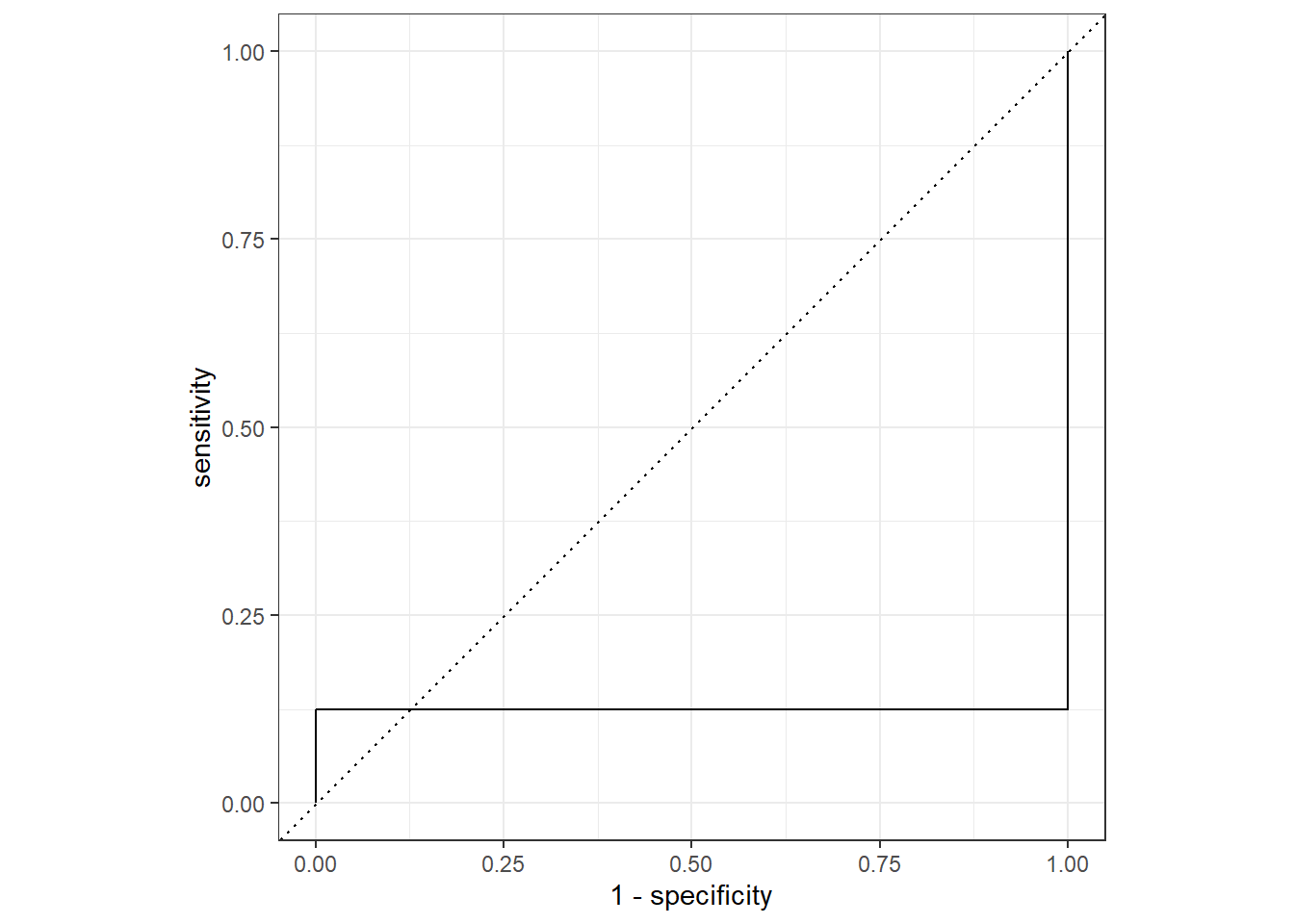

Even though my model had a decent accuracy and low Brier score during cross-validation, the ROC curve suggests it’s not reliably distinguishing between the two species. The curve stays close to the bottom and only rises at the very end, meaning it struggles to correctly identify Farinosa across most thresholds. This shows that my model may be biased toward predicting Californica and highlights a limitation in its classification performance.

Earlier, the confusion matrix showed that 3 Farinosa flowers were incorrectly predicted as Californica, and 1 Californica flower was incorrectly predicted as Farinosa. These misclassifications might happen because some flowers from the two species share similar traits, making them hard to tell apart based only on the measured variables. Also, since we only had about 100 observations, the model might not have seen enough data to learn all the patterns needed to generalize well.

In conclusion, while I was able to build and evaluate several models to classify the two Encelia species, the predictive performance was limited. The best model showed some ability to distinguish between species, but overall accuracy and the ROC analysis suggest it is not reliable for confident predictions. This outcome highlights the challenge of classifying species with overlapping traits and limited data. Future work could explore collecting more samples, incorporating additional or different traits, or trying more complex modeling techniques to improve classification accuracy.