Rent in Southern California

Objective

My goal is to take a broad look at the rental market across these Southern California counties. I want to explore what each county offers in terms of rent and identify any trends that emerge from the listings. Specifically, I’m interested in how different priorities (square footage, number of bedrooms and bathrooms, or overall price) affect where someone might choose to rent.

I understand that preferences vary, so rather than claiming one county is “best,” my goal is to highlight the trends I observe in each area and offer insights into what renters might expect based on their needs.

Packages Used and Data Import

library(readr)
library(dplyr)
library(stringr)
library(tidyverse)
library(janitor)
library(gt)
library(scales)
library(broom)
here::i_am("SoCalRentProject.qmd")
SoCalRent <- read_csv(here::here("ProjectData/SoCalDataRaw_2025.csv"))

Data Collection

Finding clean and usable public data turned out to be more challenging than expected. After exploring several sites, I’ve decided to use Redfin. I then relied on Excel’s web tools to auto-generate tables directly from listing URLs. For each listing, I’ve included the Price($), Numbers of Bathrooms and Bedrooms, Square Footage, Address, Housing Type, and County. I focused on three Southern California counties: Orange County(OC), Riverside County(RIV), and Los Angeles County(LA). Across the three counties, I gathered data on three different property types: houses, condos, and apartments. While the raw data I pulled was relatively structured, it still required some cleaning.

SoCalRent |>
  head() |>
  gt() |>
  tab_header(
    title = "Sample of Rent Listings Data"
  ) |>
  cols_label(
    Price = "Rent ($)",
    Beds = "Bedrooms",
    Baths = "Bathrooms",
    SqFt = "Square Footage",
    Address = "Address",
    Type = "Housing Type",
    County = "County"
  ) |>
opt_stylize(style = 6, color = "cyan") |>
  tab_options(
    table.font.size = px(16),
    heading.title.font.size = px(18),
    table.width = pct(100))

Sample of Rent Listings Data
Rent ($)	Bedrooms	Bathrooms	Square Footage	Address	Housing Type	County
$3,195/mo	4 beds	2.5 baths	1668.00	4001 Landau Ct, Riverside, CA 92501	house	RIV
$4,000/mo	4 beds	2 baths	2200.00	18590 Roberts Rd, Riverside, CA 92508	house	RIV
$2,300/mo	2 beds	1 bath	900.00	3468 Wallace St, Jurupa Valley, CA 92509	house	RIV
$3,449/mo	3 beds	2.5 baths	1,970	531 Atwood Ct, Riverside, CA 92506	house	RIV
$1,850/mo	1 bed	1 bath	400	2767 Attenborough Dr, Riverside, CA 92503	house	RIV
$1,950/mo	1 bed	1 bath	440	10671 Sagittarius Dr, Riverside, CA 92503	house	RIV

Data Wrangling

There were a few listings with missing data in certain columns, so for the sake of sanity, I just removed them.

Price came in various formats (e.g., $3,185/mo, $1940+/mo), so I removed dollar signs, commas, and plus signs, then converted the column to numeric.

Beds and Baths also had inconsistent formats like 1 bed, 3 beds, or even ranges like 2–4 beds. I stripped out the words “bed(s)” and “bath(s)”, and for ranges, I took the smallest number. Both columns were then converted to numeric.

SqFt was the messiest. It appeared as 1668.00, 1,970, or ranges like 410–480. I removed commas and decimal points (since I didn’t need the .00), and again, for ranges, I used the lower bound. This column was also converted to numeric.

For the address column, I kept it in case I wanted to refer to the full address later. But I also extracted just the city name into a separate column in case I wanted to analyze trends by city.

Lastly, I removed any listings where either Beds or Baths were equal to zero. This may affect apartment listing as it would have removed any studios that don’t have bedrooms.

After cleaning, I was left with 278 observations out of the original 333.

Rent_Clean <- SoCalRent |>
  #cleaning out any listings that have any empty data for the sake of my sanity
  filter(!is.na(Price), !is.na(Beds), !is.na(Baths), !is.na(SqFt), !is.na(Address), !str_starts(SqFt, "—")) |>
  mutate(
  # Price column: remove any $, +, /mo and change it to a numeric variable
  Price = str_remove_all(Price, "\\$|,|/mo|\\+"),
  Price = as.numeric(Price),
  # Beds column: take the smallest number of beds and change it to a numeric variable
  Beds = str_extract(Beds, "^\\d+"),
  Beds = as.numeric(Beds),
  # Baths column: take the smallest number of baths and change it to a numeric variable
  Baths = str_extract(Baths, "^\\d+(\\.\\d+)?"),
  Baths = as.numeric(Baths),
  # SqFt column: takeing the first number from ranges, removes and commas or dashes and change it to a numeric variable
  SqFt = str_remove_all(SqFt, ","),  # Remove commas
  SqFt = case_when(str_detect(SqFt, "-") ~ as.numeric(str_extract(SqFt, "^[0-9]+")), TRUE ~ as.numeric(SqFt)),
  # City Column: I decided to just make a new column "City"
  City = str_split_fixed(Address, ",", 3)[, 2]
  ) |>
  # If beds or baths is 0, remove the row
  filter(Beds != 0, Baths != 0)

Rent_Clean |>
  head() |>
  gt() |>
  tab_header(
    title = "Sample of Clean Rent Listings Data"
  ) |>
  cols_label(
    Price = "Rent ($)",
    Beds = "Bedrooms",
    Baths = "Bathrooms",
    SqFt = "Square Feet",
    Address = "Address",
    Type = "Housing Type",
    County = "County",
    City = "City"
  ) |>
opt_stylize(style = 6, color = "cyan") |>
  tab_options(
    table.font.size = px(16),
    heading.title.font.size = px(18),
    table.width = pct(100))

Sample of Clean Rent Listings Data
Rent ($)	Bedrooms	Bathrooms	Square Feet	Address	Housing Type	County	City
3195	4	2.5	1668	4001 Landau Ct, Riverside, CA 92501	house	RIV	Riverside
4000	4	2.0	2200	18590 Roberts Rd, Riverside, CA 92508	house	RIV	Riverside
2300	2	1.0	900	3468 Wallace St, Jurupa Valley, CA 92509	house	RIV	Jurupa Valley
3449	3	2.5	1970	531 Atwood Ct, Riverside, CA 92506	house	RIV	Riverside
1850	1	1.0	400	2767 Attenborough Dr, Riverside, CA 92503	house	RIV	Riverside
1950	1	1.0	440	10671 Sagittarius Dr, Riverside, CA 92503	house	RIV	Riverside

Exploratory Data Analysis

I analyzed the data by grouping listings by County and Housing Type.

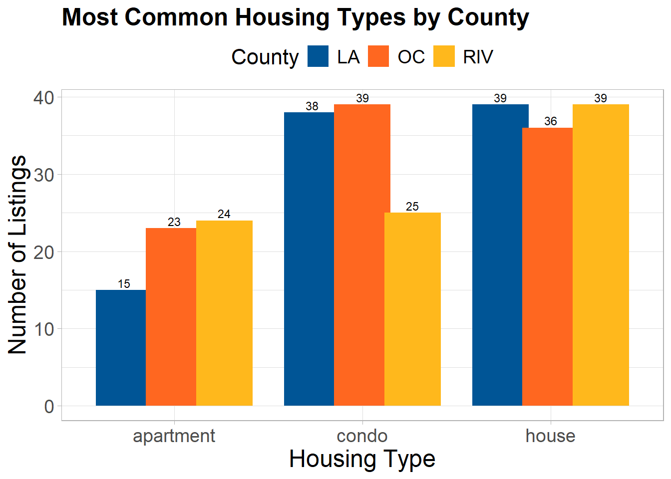
Overall, most listings were houses. Riverside County had the highest number of apartment listings, while Orange County had the most condo listings. When it comes to house listings, Riverside and Los Angeles counties were tied for the highest count.

Rent_Clean |>
  count(Type, County) |>
  ggplot(aes(x = Type, y = n, fill = County)) +
  geom_bar(stat = "identity", position = position_dodge(width = 0.8)) +
  geom_text(aes(label = n), 
            position = position_dodge(width = 0.8), 
            vjust = -0.3, size = 3) +
  scale_fill_manual(
  values = c("LA" = "#005596", "OC" = "#FF6720", "RIV" = "#FFB81C")
)+
  labs(
    title = "Most Common Housing Types by County",
    x = "Housing Type", 
    y = "Number of Listings"
  ) +
  theme_light() +
  theme(
    legend.position = "top",
    text = element_text(size = 16),             
    axis.title = element_text(size = 18),        
    axis.text = element_text(size = 14),         
    plot.title = element_text(size = 18, face = "bold"),
    legend.title = element_text(size = 16),     
    legend.text = element_text(size = 14)   
  )

Next, I made a table showing the average and median rent prices by county and housing type. As expected, apartments were the most affordable option across all counties, with Riverside having the lowest average price. On the other end, houses in Orange County stood out as the most expensive, with an average rent of $7,388. Condo prices varied widely, suggesting a mix of both luxury and more affordable units across different areas.

It was important to notice the difference between average and median values. This indicates that there exists high-priced outliers that are skewing the averages. Median values offer a better sense of typical rent prices.

summary_table <- Rent_Clean |>
  group_by(County, Type)|>
  summarize(mean.price = round(mean(Price, na.rm = TRUE)), 
            median.price = median(Price, na.rm = TRUE),
            .groups = "drop")
summary_table |>
  arrange(desc(mean.price))|>
  gt() |>
  tab_header(
    title = "Average Rent Price by County and Type") |>
  fmt_currency(
    columns = c(mean.price, median.price),
    currency = "USD",
    decimals = 0) |>
  cols_label(
    County = "County",
    Type = "Housing Type",
    mean.price = "Average Rent",
    median.price = "Median Price") |>
  data_color(
    columns = c(mean.price),
    colors = col_numeric(
      palette = c(palette = c("#2ecc71", "#f1c40f", "#e74c3c")),
      domain = NULL
    )
  ) |>
  cols_align(align = c("left"))|>
  opt_stylize(style = 6, color = "gray") |>
  tab_options(
    table.font.size = px(16),
    heading.title.font.size = px(20),
    heading.subtitle.font.size = px(14),
    data_row.padding = px(3),
    table.width = pct(100))

Average Rent Price by County and Type
County	Housing Type	Average Rent	Median Price
OC	house	$7,388	$6,850
LA	house	$6,547	$5,995
OC	condo	$4,385	$4,000
LA	condo	$3,673	$3,500
LA	apartment	$3,525	$2,950
RIV	house	$3,169	$3,400
OC	apartment	$2,595	$2,535
RIV	condo	$2,479	$2,400
RIV	apartment	$1,885	$1,865

To better visualize the distribution of rent prices and identify outliers, I created a boxplot grouped by County and Housing Type. The red dots represent outlier listings, which are values that fall significantly above the average rent range.

This visualization shows that Orange County and Los Angeles have several high-priced outliers, particularly for houses and condos. These extreme values help explain why the average rent is much higher than the median in those areas.

Rent_Clean |> 
  ggplot(aes(x = Type, y = Price, fill = County)) +
  geom_boxplot(outlier.shape = 16, outlier.colour = "#e74c3c", outlier.size = 3) +
  labs(
    title = "Rent Price Distribution by County and Housing Type",
    x = "County",
    y = "Rent Price ($)"
  ) +
  scale_fill_manual(
    values = c("LA" = "#005596", "OC" = "#FF6720", "RIV" = "#FFB81C")
  ) +
  scale_y_continuous(trans = "log10") +  # Log scale to reduce skew
  theme_light() +
  theme(
    legend.position = "top",
    text = element_text(size = 16),             
    axis.title = element_text(size = 18),        
    axis.text = element_text(size = 14),         
    plot.title = element_text(size = 16, face = "bold"),
    legend.title = element_text(size = 16),     
    legend.text = element_text(size = 14)   
  )

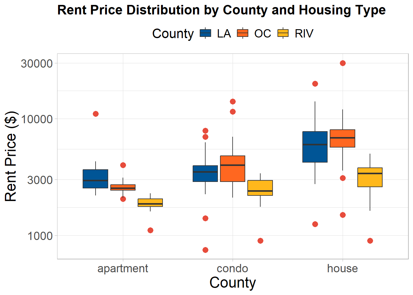
These patterns in the number of listings and rent prices reveal the differences in the housing market across Southern California. Riverside’s high number of apartment listings and lower average rents point to its role as a more affordable and accessible housing market. Riverside has few outliers, suggesting more consistency in pricing and older/cheaper properties.

In contrast, Los Angeles and Orange County show multiple high-end outliers, especially for houses and condos, which increase the average prices. These outliers hint at the presence of luxury markets or high-demand neighborhoods.

How to define what gets filtered

For this project, I want to approach rental affordability from a personal angle, while keeping it general enough that others could adapt it to their own situations. A common rule of thumb is that individuals shouldn’t spend more than 30% of their income on rent. Based on this, I’ll introduce a salary variable to simulate what someone can realistically afford. This variable will help filter out listings that exceed that 30% income threshold.

To make the analysis more flexible, especially for listings with multiple bedrooms, I’m assuming that shared housing is an option. That means I’ll consider a unit affordable if the rent per bedroom is within 30% of a person’s monthly income. This way, I can include multi-bedroom housing options that might be affordable when split among roommates.

salary <- 60000  # random yearly salary
monthly_income <- salary / 12 #calculating monthly paycheck assuming monthly rent payments
max_rent <- (monthly_income * 0.30) #only 30% of income to be used for rent
Rent_Clean_Affordable <- Rent_Clean |> #filter out to only include the affordable listings
  mutate(
    rent_per_room = Price / Beds, #allowing for roomates
    affordable = rent_per_room <= max_rent #makes logical
  )|>
  filter(affordable== TRUE) #filter
summary_affordable <- Rent_Clean_Affordable |> #making a new mean/median table but consider affordability
  group_by(County, Type)|>
  summarize(mean.price = round(mean(Price, na.rm = TRUE)), 
            median.price = median(Price, na.rm = TRUE),
            .groups = "drop")
summary_affordable |> #make a new visually appealing table
  arrange(desc(mean.price))|>
  gt() |>
  tab_header(
    title = "Average Rent Price by County and Type") |>
  fmt_currency(
    columns = c(mean.price, median.price),
    currency = "USD",
    decimals = 0) |>
  cols_label(
    County = "County",
    Type = "Housing Type",
    mean.price = "Average Rent",
    median.price = "Median Price") |>
  data_color(
    columns = c(mean.price),
    colors = col_numeric(
      palette = c(palette = c("#2ecc71", "#f1c40f", "#e74c3c")),
      domain = NULL
    )
  ) |>
  cols_align(align = c("left"))|>
  opt_stylize(style = 6, color = "gray") |>
  tab_options(
    table.font.size = px(16),
    heading.title.font.size = px(20),
    heading.subtitle.font.size = px(14),
    data_row.padding = px(3),
    table.width = pct(100))

Average Rent Price by County and Type
County	Housing Type	Average Rent	Median Price
LA	house	$4,360	$4,400
OC	house	$4,211	$4,098
OC	condo	$3,630	$3,958
RIV	house	$3,369	$3,450
LA	condo	$3,276	$3,500
LA	apartment	$2,970	$2,798
OC	apartment	$2,775	$2,775
RIV	condo	$2,568	$2,542
RIV	apartment	$1,926	$1,950

After adding the salary variable, I was able to realistically filter out the extreme outliers. After removing these high rent listings the average rent moved closer to the median. This suggests that the original averages were heavily influenced by a small number of expensive listings.

This adjustment is especially important for model building. By filtering out outliers, we create a dataset that better represents the usual trends, making our model more reliable.

Multiple Linear Regression Model

I made a multiple linear regression model to analyze how rent prices in Southern California are influenced by factors including county, housing type, number of bedrooms, bathrooms, and square footage. The model reveals several important relationships.

rent_model <- lm(Price ~ County + Type + SqFt + Beds + Baths, 
                 data = Rent_Clean_Affordable) #the model :D
rent_model_table <- rent_model |> tidy() #the model into table

rent_model_table <- rent_model_table |> #mutate p.val to highlight significance
  mutate(p.value = case_when(
    p.value <= 0.05 ~ "≤ 0.05",    # Highly significant
    p.value > 0.05 ~ "> 0.05",     # Non-significant
    TRUE ~ as.character(p.value)
  ),
  Change_Price = case_when( #highlight changes in price
    estimate > 0 ~ "increase",  # Positive coefficient (increase)
    estimate < 0 ~ "decrease",  # Negative coefficient (decrease)
    TRUE ~ "neutral"            # Neutral
  ))

rent_model_table |> #make pretty table
  gt() |>
  tab_header(
    title = "Regression Results for Rent Model"
  ) |>
  cols_label(
    term = "Variable",
    estimate = "Estimate",
    std.error = "Standard Error",
    statistic = "t-Statistic",
    p.value = "p-Value",
    Change_Price = "Change in Price"
  ) |>
  tab_spanner(
    label = "Coefficients",
    columns = c(estimate, std.error, statistic, p.value)
  ) |>
  tab_style(
    style = cell_text(color = "#2ecc71"),
    locations = cells_body(columns = vars(estimate), 
                           rows = Change_Price == "increase")
  ) |>
  tab_style(
    style = cell_text(color = "#e74c3c"),
    locations = cells_body(columns = vars(estimate), 
                           rows = Change_Price == "decrease")
  ) |>
    tab_style(
    style = cell_text(color = "#e74c3c"),
    locations = cells_body(columns = vars(p.value), 
                           rows = p.value == "> 0.05") #heavy sig
  ) |>
  tab_style(
    style = cell_text(color = "#2ecc71"),
    locations = cells_body(columns = vars(p.value),  #non sig
                           rows = p.value == "≤ 0.05")
  ) |>
   cols_align(align = c("left"))|>
opt_stylize(style = 6, color = "gray") |>
  tab_options(
    table.font.size = px(16),
    heading.title.font.size = px(18),
    table.width = pct(100))

Regression Results for Rent Model
Variable	Coefficients				Change in Price
	Estimate	Standard Error	t-Statistic	p-Value
(Intercept)	1028.1934539	219.212166	4.6904032	≤ 0.05	increase
CountyOC	188.9374670	143.341713	1.3180913	> 0.05	increase
CountyRIV	-718.4149778	111.538787	-6.4409431	≤ 0.05	decrease
Typecondo	73.2123135	172.780024	0.4237314	> 0.05	increase
Typehouse	401.2195019	188.448517	2.1290669	≤ 0.05	increase
SqFt	-0.1666292	0.155018	-1.0749019	> 0.05	decrease
Beds	844.4871509	97.993519	8.6177857	≤ 0.05	increase
Baths	70.5854399	108.488020	0.6506289	> 0.05	increase

An apartment in LA is our baseline. Listings in the OC area are higher than LA (by $189) but it is not statistically significant. Listing in the Riverside area tend to cost less than in Los Angeles, this difference is statistically significant.

The number of bedrooms had the strongest and most statistically significant association with rent. Each additional bedroom increases rent by approximately $844 on average. Baths are not as statistically significant only increasing rent by $70.

Houses rent for approximately $401 more than apartments but shown by the model, doesn’t have. Condos are not statistically significant, only increasing rent by $73.

Although Square Footage is often expected to impact rent, in this model it is not accurate. Suggesting other factors may play a bigger role (i.e. bedrooms). This model can indicate that the number of bedrooms may play a more important role in rent pricing than square footage, possibly because people value how many individuals a space can house more than the size itself.

Prediction <- rent_model|>
  augment( newdata= Rent_Clean_Affordable)
# Plot the residuals
ggplot(data = Prediction, aes(x = .resid)) +
  geom_histogram(bins = 10, fill = "#005596", color = "black", alpha = 0.8) +
  labs(title = "Histogram of Residuals",
       x = "Residuals",
       y = "Frequency") +
  theme_light() +
  theme(
    legend.position = "top",
    text = element_text(size = 16),             
    axis.title = element_text(size = 18),        
    axis.text = element_text(size = 14),         
    plot.title = element_text(size = 16, face = "bold"),
    legend.title = element_text(size = 16),     
    legend.text = element_text(size = 14)   
  )

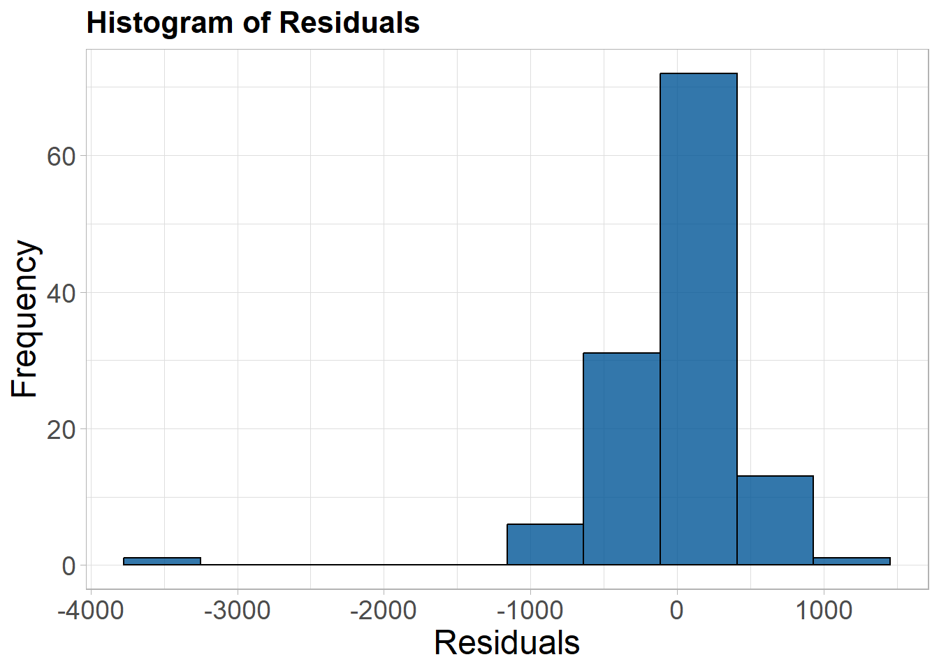
This histogram visualizes the distribution of residuals from the multiple linear regression model. The residuals are mostly centered around zero, indicating that the model generally makes accurate predictions. However, there is a slight skew to the left, suggesting that the model tends to overestimate rent prices for a number of listings.

Conclusion

After exploring the data using multiple methods, I was able to uncover key housing trends across each of the Southern California counties. As someone who has lived here for over 20 years, many of these patterns align with my lived experience but it’s pretty cool to see data analytics prove what me and other locals often see.

Los Angeles (LA):
As expected, LA is a heavily populated area and has some of the highest rent prices. The correlation analysis shows that square footage has a stronger impact on rent in LA, likely due to the high demand and limited space (many people, not much room). The histogram also reveals a right-skewed distribution, with prices trailing into the more expensive range, reinforcing the idea of LA as a competitive and costly housing market.

Riverside (RIV):
Riverside’s histogram displays lower rent values. Its status as an older, more suburban region contributes to its relative affordability. The correlation table shows a balanced influence from the number of beds, baths, and square footage on pricing. This suggests that Riverside follows more predictable pricing patterns. It reflects a suburban area offering more consistent and accessible housing options.

Orange County (OC):
Unlike LA and Riverside, Orange County’s histogram doesn’t show a clear skew, indicating a wide spread of rent prices. This suggests a mix of older, more affordable homes and newer, high-end properties. The weaker correlation between basic housing features and rent price implies that other external factors (school quality, neighborhood amenities, community in general) may play a more important role in determining rent in Orange County.

correlation_table <- Rent_Clean |>
  group_by(County) |>
  summarise(
    Bed_cor = cor(Price, Beds), 
    Baths_cor = cor(Price, Baths), 
    SqFt_cor = cor(Price, SqFt)
  )
correlation_table |>
  gt() |>
  tab_header(
    title = "Correlation of Rent Price with Features by County"
  ) |>
  cols_label(
    County = "County",
    Bed_cor = "Price vs Beds",
    Baths_cor = "Price vs Baths",
    SqFt_cor = "Price vs SqFt"
  ) |>
  tab_style(
    style = cell_text(weight = "bold"),
    locations = cells_column_labels(columns = everything())
  ) |>
   cols_align(align = c("left"))|>
opt_stylize(style = 6, color = "cyan") |>
  tab_options(
    table.font.size = px(16),
    heading.title.font.size = px(18),
    table.width = pct(100))

Correlation of Rent Price with Features by County
County	Price vs Beds	Price vs Baths	Price vs SqFt
LA	0.5704509	0.4944130	0.7294382
OC	0.4496779	0.5389367	0.5983870
RIV	0.9013643	0.7824197	0.7990179

Rent_Clean |>
  filter(Price < 10000)|>
  mutate(County = as.character(County)) |>
  bind_rows(
    Rent_Clean_Affordable |>
      mutate(County = "All Counties")
  ) |>
  ggplot(aes(x = Price, fill = County)) +
  geom_histogram(binwidth = 800, color = "black") +
  facet_wrap(~ County, scales = "free_y") +
  labs(
    title = "Rent Price Distribution: Overall and by County",
    x = "Rent Price ($)",
    y = "Number of Listings"
  ) +
  scale_fill_manual(
    values = c("LA" = "#005596", "RIV" = "#FFB81C","OC" = "#FF6720", 
      "All Counties" = "gray" 
    )
  ) +
  theme_light() +
  theme(
    text = element_text(size = 16),             
    axis.title = element_text(size = 18),        
    axis.text = element_text(size = 14),         
    plot.title = element_text(size = 16, face = "bold"),
    legend.title = element_text(size = 16),     
    legend.text = element_text(size = 14)   
  )

Which brings me back to my objective: Where should someone rent? As mentioned earlier, the answer depends on individual priorities. If you’re looking for consistent affordability, Riverside is a solid choice with its more predictable and accessible pricing. The LA area, while expensive, reflects the appeal and allure of the area beyond just housing. As for Orange County, it’s great for those seeking a balance between affordability and amenities. It offers a mix of options for people who value a comfortable lifestyle with access to good schools, parks, and community features.

Ultimately, there’s no one-size-fits-all answer. Renters must weigh their priorities, whether it’s budget, space, amenities, or proximity to work and culture, in order to find the right fit for them.

Limitations

Even though this project helped uncover some cool insights about rent trends in Southern California, there were a few limitations worth mentioning.

Data Source:
The data I used was based on the rental listings available during this time (APR 2025) and like most online listings, they change fast. Some of the ones I pulled were already taken down a couple of weeks later. On top of that, there were some missing or weird values in the dataset. For example, some listings had 0 bedrooms, which probably meant they were studios. But the way the data was structured (and for simplicity as a beginner), I chose to remove them. I remember that decision actually cut out a decent number of apartment listings from LA, which probably skewed the overall picture there a bit.

Modeling Assumptions:
I used a linear regression model, which assumes a straight-line relationship between things like square footage, beds, and baths, and the rent price. But let’s be real, housing markets are way more complicated than that. There are tons of other factors that influence rent like location, neighborhood vibe, schools, commute times and those things are hard to capture with the dataset I had. So while the model gives us a starting point, it definitely doesn’t tell the whole story.

Reflection

This project was genuinely a lot of fun. Working with real housing data pushed me to practice key skills like data cleaning and wrangling. I felt way more confident in organizing messy data and turning it into something meaningful. I especially enjoyed creating the visuals and being able to actually see the trends and share them in a clear way.

I also connected with this project on a personal level. I’ve lived in Southern California my whole life, so it was really interesting to analyze an everyday topic like rent through the lens of a data analyst. It helped me understand how prices vary and what factors play a role in shaping the housing landscape across different counties.

There were definitely a few more things I would’ve liked to explore or experiment with, but I decided to focus on cleaning and improving the work I already had. Honestly, just being able to turn data into visuals and insights was exciting enough.

EXTRA: my favorite weird listings

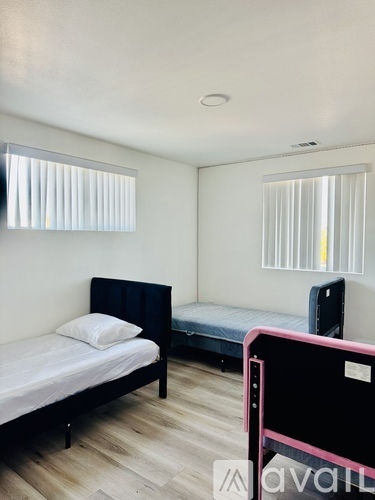
217 E 29th St Unit 217 and 217 1/2, Los Angeles, CA 90011: Upon further investigation, this is actually a listing for two units with a total of 4 beds and 4 baths—so 2 beds and 2 baths per unit. The listing also mentions that each bedroom can house 2–3 people. Based on how my code calculates rent per person, that would come out to around $187/month, give or take a roommate or two.

As amazing as that rent price sounds, it definitely raises some eyebrows. On the bright side, it could be a legit affordable housing option for someone who really needs it. But on the more skeptical side… the listing gives off some sketchy vibes. Personally, I’m not interested.

Rental Description: Our brand new, all-inclusive shared rooms are move-in ready just bring your bag and settle into comfort, convenience, and community in the heart of the city. All-inclusive rates starting at just $700/month only 2-3 person per room ! Move in today stay as long or as little as you need All utilities Wi-Fi included Weekly cleaning of shared spaces Private ensuite bathrooms in most rooms On-site laundry for easy living Street & paid parking available On-site manager for support when you need it No credit checks. No deposits. No SSN. Just a valid ID from any country.Spots are limited and going fast message now and claim your bed today!”

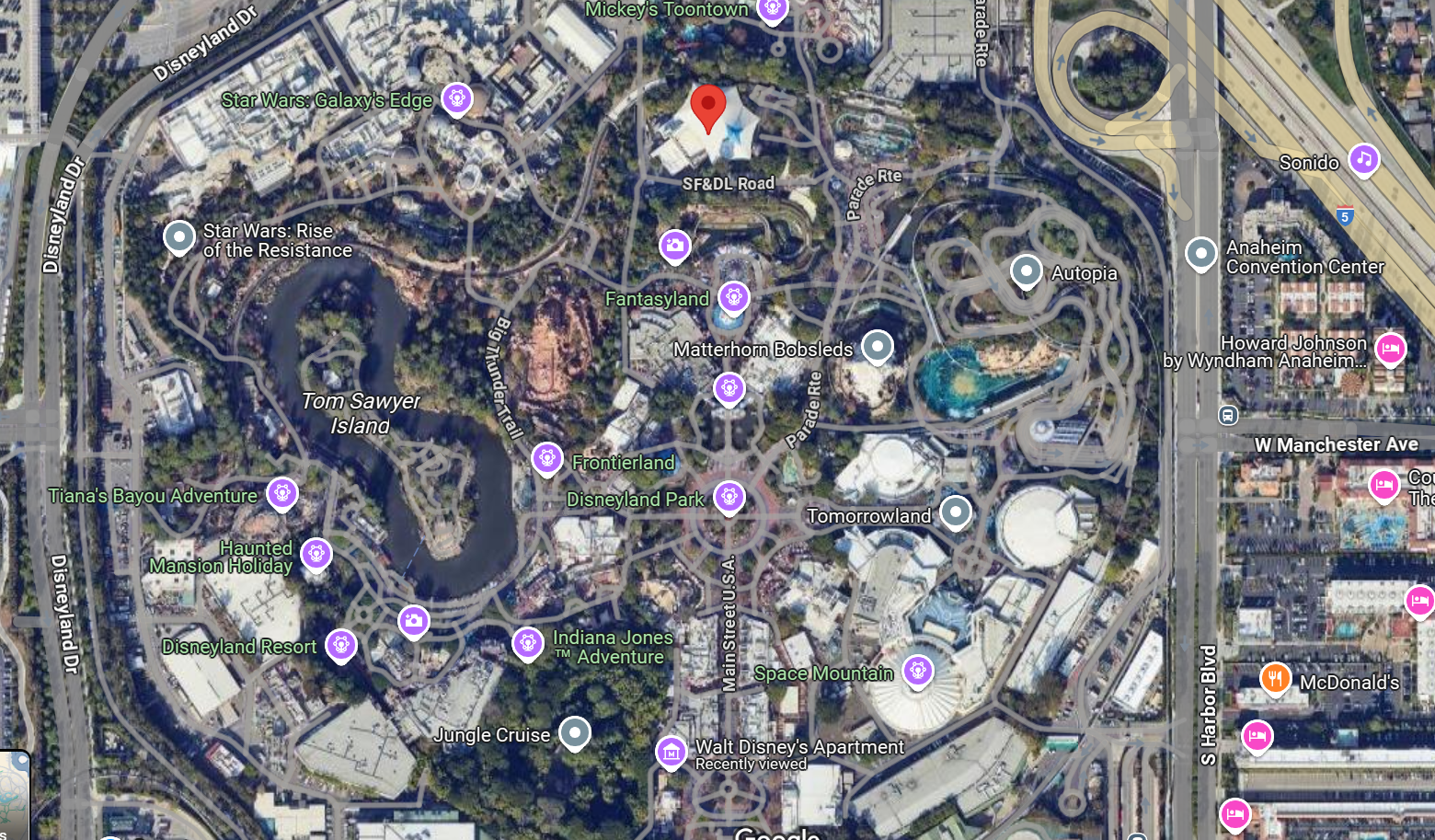
1313 Disneyland Dr., Anaheim, CA 92802: This listing was up for rent at $30,000/month and completely skewed my average rental price for Orange County. At first, I assumed it was just a fancy condo near Disneyland. But when I looked into it, I realized it was actually inside Disneyland. Weird.

Curious (and knowing there are plenty of Disneyland superfans out there), I searched Reddit and sure enough, 1313 Disneyland Dr. is the park’s official address. Fun fact: M is the 13th letter of the alphabet, so 1313 = MM = Mickey Mouse. I couldn’t find much else about what this listing actually was.

The listing had been up for nearly a year and only got taken down recently on April 30th, 2025. My best guess? Maybe it was the apartment above the fire station that Walt Disney supposedly used. But more realistically, it could’ve been something related to private entertainment or internal use within Disneyland.

Still, kind of strange that the listing disappeared just two weeks after I pulled the data.

Rental Description: This property is available. Please inquire on this site to schedule a showing. Im sorry, I cant provide a description of this property.Available NOWHeating ForcedAirCooling EvaporativeAppliances Refrigerator, Range Oven, Microwave, DishwasherLaundry In UnitParking Detached Garage, 2 spacesPets Dogs Allowed, Cats AllowedSecurity deposit 30,000.00Included Utilities Garbage, Sewage, LandscapingAdditional DepositPet 500.00This property has a home security system.Disclaimer Ziprent is acting as the agent for the owner. Information Deemed Reliable but not Guaranteed. All information should be independently verified by renter.