Covid Lung Capacity Analysis

Math 439 HW 1
Natalie Torres
Note: Worked with Ashley on the code :)

Introduction

We are analyzing whether vaccinated individuals have higher lung capacity after contracting Covid compared to unvaccinated individuals.

In the data given, lung capacity is measured on a scale from 0–100. The control group consists of individuals who contracted Covid and were unvaccinated, while the vaccinated group received the vaccine before getting Covid.

Data Loading

covid <- read.csv("Instruction_Data/covid.csv")
control <- covid$control
vaccinated <- covid$vaccinated
# control: individuals who contracted virus and no vaccine
# vaccinated: individuals who took vaccine then got Covid

PART A: Two-sample t-test

We’re concernced about whether or not vaccinated individuals have a have a higher lung capacity compared to unvaccinated individuals. Let H₀ be the null hypothesis that unvaccinated individuals have the same average lung capacity as vaccinated individuals.

# parameters
c.x.bar <- mean(control)
v.x.bar <- mean(vaccinated)
obs.diff <- v.x.bar - c.x.bar # needed later for simulation

s.control <- sd(control)
s.vaccinated <- sd(vaccinated)

n <- length(control)

# t-test (one-sided, greater)
t.test(vaccinated, control, alternative="greater")

    Welch Two Sample t-test

data:  vaccinated and control
t = 3.4094, df = 398, p-value = 0.0003588
alternative hypothesis: true difference in means is greater than 0
95 percent confidence interval:
 4.258564      Inf
sample estimates:
mean of x mean of y 
 63.01579  54.76957 

The result of our two-sample t-test shows that the p-value = 0.0003588 (less than 0.05), we reject the null hypothesis that the group averages are equal. Thus, the average lung capacity in the vaccinated group is higher than in the control group.

PART B: Bootstrapping

Not convinced? We can run a simulation 10,000 times to determine if we get the same outcome for more then the just the sample size we have.

set.seed(42)
# Histograms
# hist(control, breaks = 5)
# hist(vaccinated, breaks = 5)

# Recenter to make H0 true (both means equal)
control.pseudo.pop <- control - mean(control) + 50
vaccinated.pseudo.pop <- vaccinated - mean(vaccinated) + 50

# 10000 simulations for control
c.sim.xbars = rep(0,10000)
for(i in 1:10000){
  c.sim.xbars[i] = mean(sample(control.pseudo.pop,n,replace=T))
}

# 10000 simulations for vaccinated
v.sim.xbars = rep(0,10000)
for(i in 1:10000){
  v.sim.xbars[i] = mean(sample(vaccinated.pseudo.pop,n,replace=T))
}
# Simulated differences
sim.diff = v.sim.xbars - c.sim.xbars

# Plot
hist(sim.diff, breaks = 20,
     main = "Histogram of Bootstrap",
     xlab = "Difference in Means (Vaccinated − Control)")
lines(c(obs.diff, obs.diff), c(0, 10000), col = 2, lty = 2)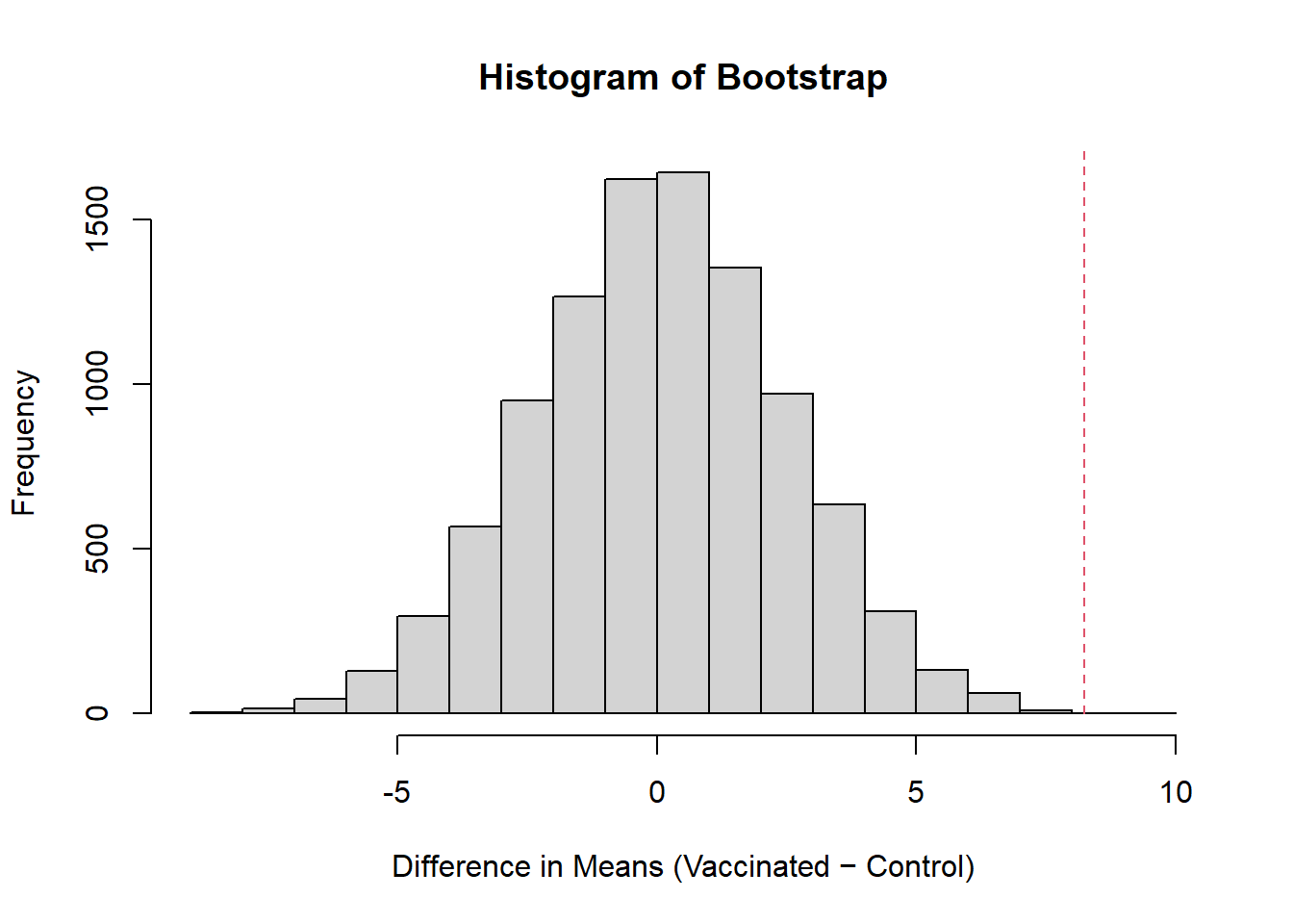

# Simulated p-val
sim.pval = length(sim.diff[sim.diff>obs.diff])/10000
sim.pval

[1] 3e-04

In this histogram, the red dashed line shows the difference we actually observed. Because it’s way out on the edge we can reject the null hypothesis (H₀).

The two-sample t-test and the bootstrap simulation both assess whether the vaccinated group has higher mean lung capacity than the control group. The t-test gave a p-value of 0.00036, while the bootstrap gave a p-value of 0.0003. Both results indicate that vaccinated individuals have a higher lung capacity. Getting the same p-value from both method methods, further solidifies this claim.

PART C: Bootstrapping the 10th Percentile

Consider the idea that we may want to look at the worse cases. So we take the 10th percentile of both groups and compare them.

set.seed(42)
# Observed 10th percentile difference
p10.obs.diff <- quantile(vaccinated, 0.10) - quantile(control, 0.10)

# 10000 simulations for control
c10.sim.xbars = rep(0,10000)
for(i in 1:10000){
  c10.sim.xbars[i] = quantile(sample(control.pseudo.pop,n,replace=T),0.10)
}

# 10000 simulations for vaccinated
v10.sim.xbars = rep(0,10000)
for(i in 1:10000){
  v10.sim.xbars[i] = quantile(sample(vaccinated.pseudo.pop,n,replace=T),0.10)
}

# Simulated difference
p10.sim.diff = v10.sim.xbars - c10.sim.xbars

# Plot
hist(p10.sim.diff,breaks=20,
     main = "Histogram of Bootstrap 10th Percentile",
     xlab = "Difference in Means (Vaccinated − Control)")
lines(c(p10.obs.diff,p10.obs.diff),c(0,10000),col=2,lty=2)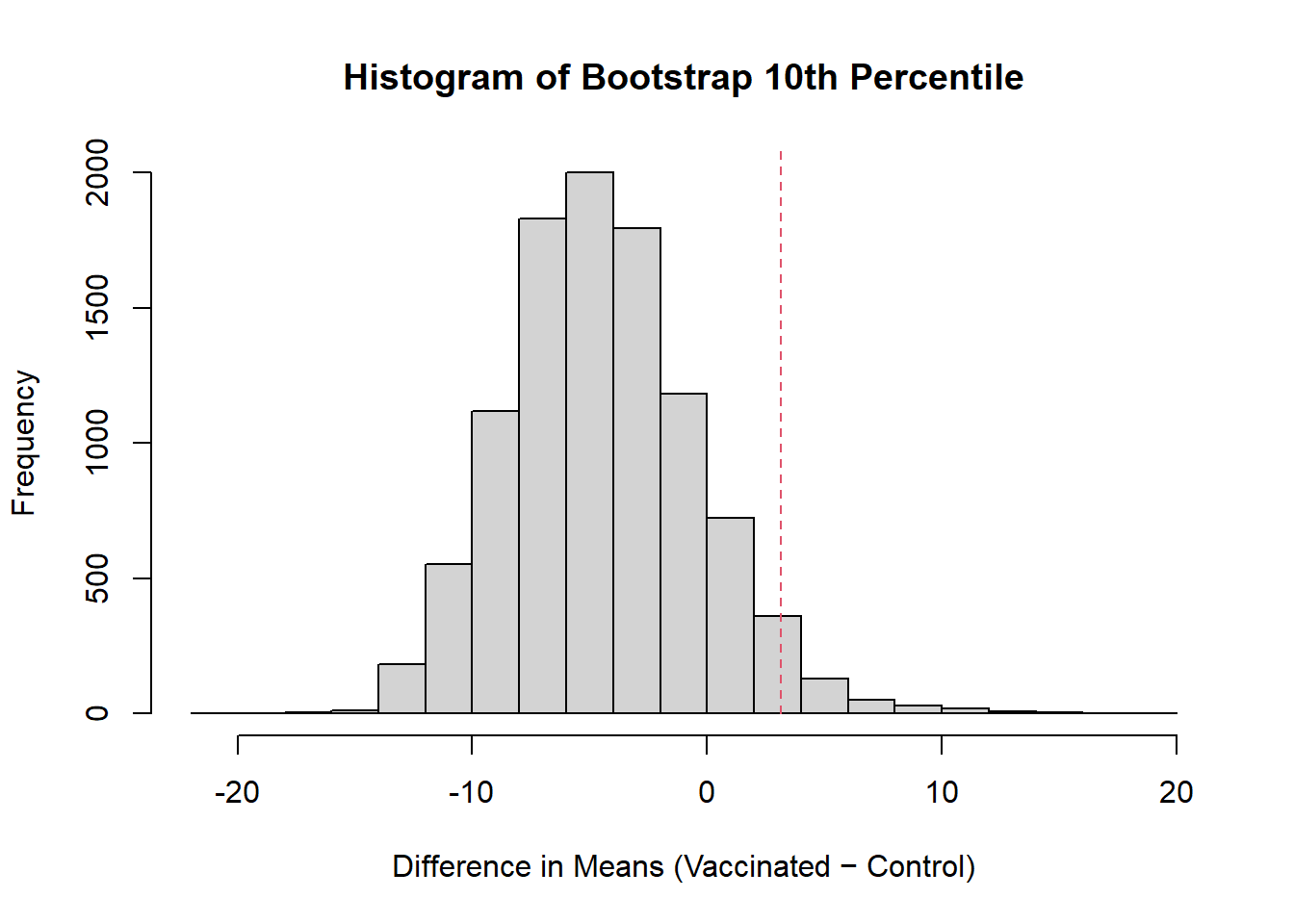

p10.sim.pval = length(p10.sim.diff[p10.sim.diff>p10.obs.diff])/10000
p10.sim.pval

[1] 0.0367

Since the p-value is for the 10th percentile is 0.0367 this means that the lowest lung capacities in the vaccinated group are likely higher than those in the control group and is not just random. Meaning even at their worst, vaccinated individuals tend to have better lung capacities than the control group.

Part D: Bias Discussion

It’s important to acknowledge that Part C can be biased. The sample we have is only a subset of the population, so it could contain more low or high values than the population. This means the 10th percentile we calculated here could overestimate or underestimate the true population 10th percentile.

Using the mean can be more reliable, since it uses all values rather than focusing on extremes. If we do want to use percentiles, it’s helpful to report confidence intervals and consider other percentiles as well. That way we can show whether the observed 10th percentile is part of a consistent trend or just due to sampling variability.

Conclusion

The analysis suggests that vaccinated individuals tend to have higher lung capacities than the control group. This indicates that the antibodies developed from vaccination may help maintain healthier lungs even when infected with Covid.