Earthquake Relationships

This project analyzes earthquake mainshocks and their aftershocks using a dataset collected from the Atacama Fault Zone.

library(readr)
library(ggplot2)

Warning: package 'ggplot2' was built under R version 4.4.3

midterm1 <- read_csv("midterm1.csv")

Rows: 110 Columns: 2
── Column specification ────────────────────────────────────────────────────────
Delimiter: ","
dbl (2): aftershock, mainshock

ℹ Use `spec()` to retrieve the full column specification for this data.
ℹ Specify the column types or set `show_col_types = FALSE` to quiet this message.

# residual diagnositics with no transformation
x= midterm1$mainshock
y= midterm1$aftershock

model = lm(y~x)
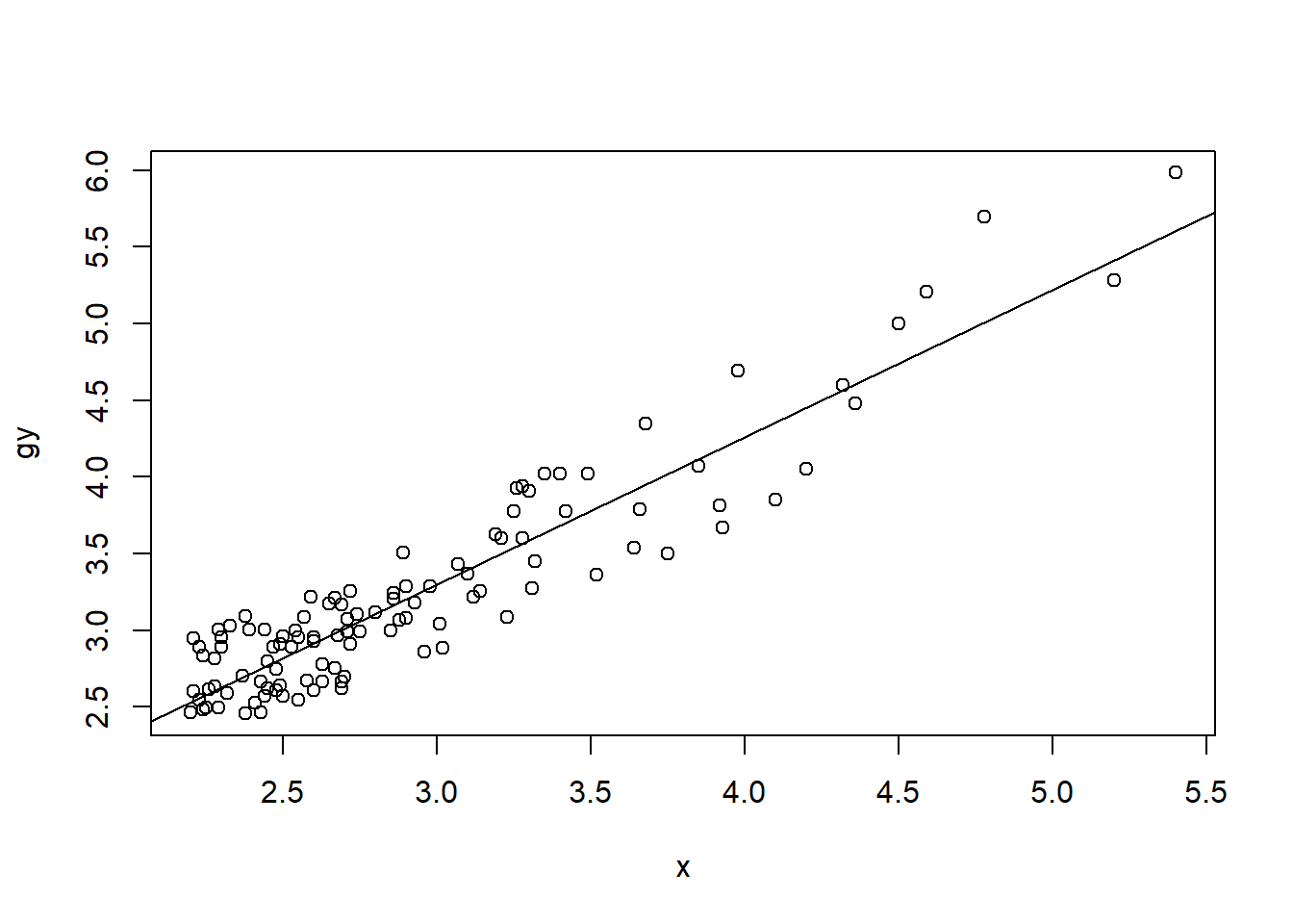
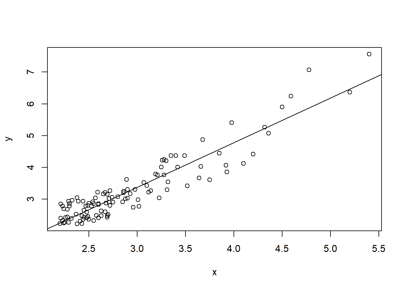
plot(x,y)
abline(lm(y~x))

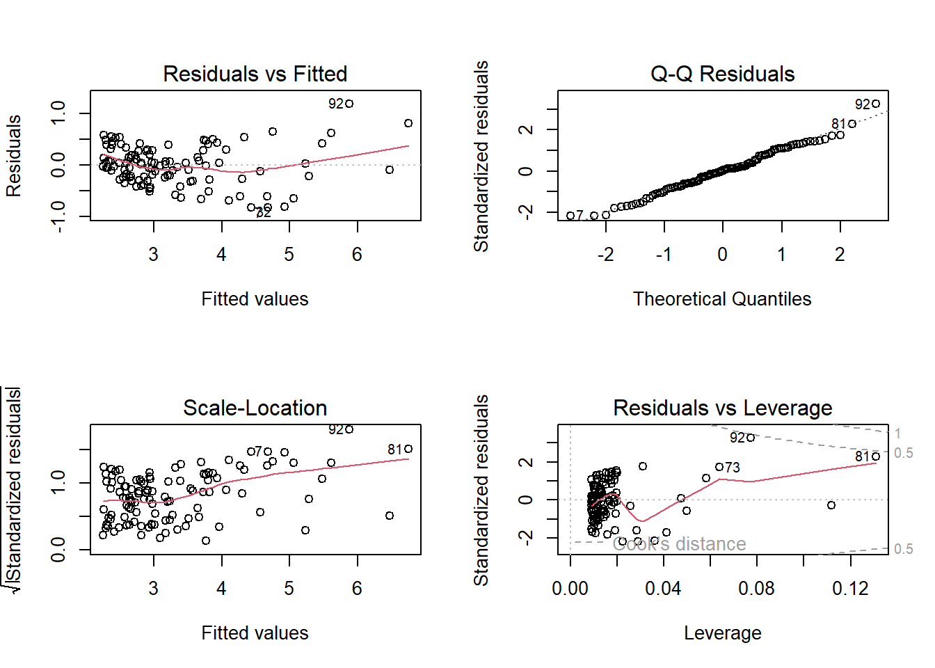
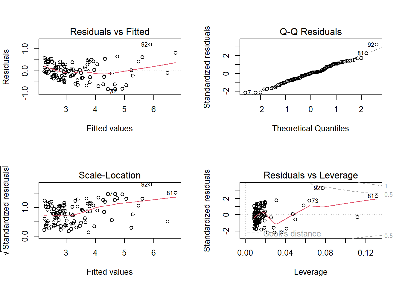
par(mfrow=c(2,2))
plot(model)

lam is 0.73

#transforming y
trans.y = function(lambda){
    gy = (y^lambda - 1)/lambda
    SSR = sum((lm(x~gy)$residuals)^2)
    SSR
}

lam = optim(1,trans.y)$par

Warning in optim(1, trans.y): one-dimensional optimization by Nelder-Mead is unreliable:
use "Brent" or optimize() directly

gy = (y^lam)/lam
plot(x,gy)
abline(lm(gy~x))

lam

[1] 0.7261719

model1 = lm(y~x)
par(mfrow=c(2,2))
plot(model1)

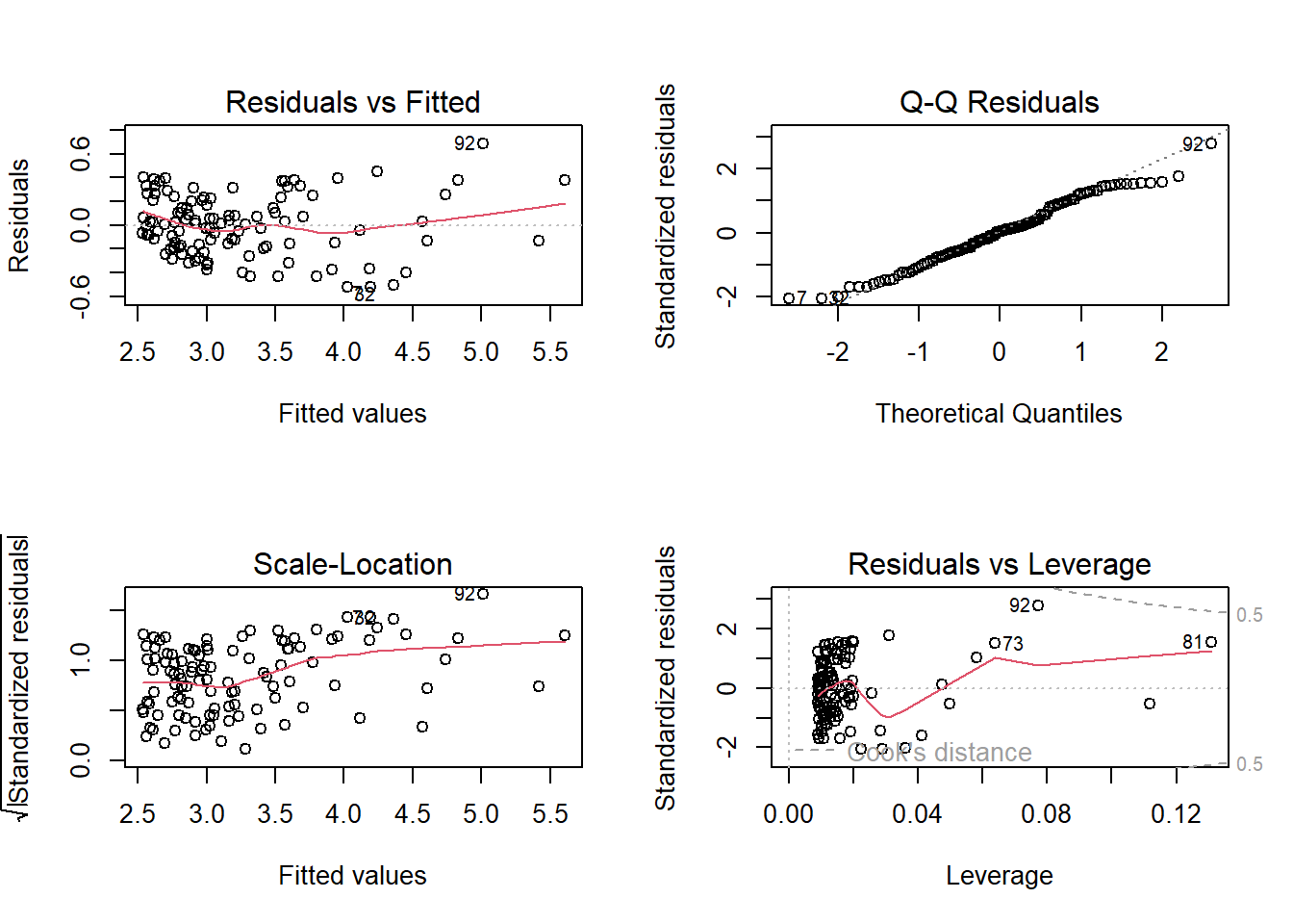
model2 = lm(gy~x)
par(mfrow=c(2,2))
plot(model2)

STEP A

The intercept is .42: predicts a slight positive aftershock after mainshock mag is 0

Slope is .96: for every 1 mag increase in mainshock the aftershock inscrease by .96 Showing a strong pos relationship.

P-val is 2.2e-16 meaning the positive relationship isnt something random

R^2: 86%. very strong. showing aftershock mag are can heavily be predicted by the mainshock mag

Residuals show that linear model is reasonable and no transformation is needed.
IE: bigger earthquakes have bigger aftershocks

# Load data
x <- midterm1$mainshock
y <- midterm1$aftershock
#transforming y
trans.y = function(lambda){
    gy = (y^lambda - 1)/lambda
    SSR = sum((lm(x~gy)$residuals)^2)
    SSR
}

lam = optim(1,trans.y)$par

Warning in optim(1, trans.y): one-dimensional optimization by Nelder-Mead is unreliable:
use "Brent" or optimize() directly

gy <- (y^lam - 1) / lam
model_bc <- lm(gy ~ x)
summary(model_bc)

Call:
lm(formula = gy ~ x)

Residuals:
     Min       1Q   Median       3Q      Max 
-0.52350 -0.17697  0.00849  0.21145  0.68690 

Coefficients:
            Estimate Std. Error t value Pr(>|t|)    
(Intercept) -0.96201    0.11021  -8.729 3.55e-14 ***
x            0.96168    0.03657  26.297  < 2e-16 ***
---
Signif. codes:  0 '***' 0.001 '**' 0.01 '*' 0.05 '.' 0.1 ' ' 1

Residual standard error: 0.258 on 108 degrees of freedom
Multiple R-squared:  0.8649,    Adjusted R-squared:  0.8637 
F-statistic: 691.5 on 1 and 108 DF,  p-value: < 2.2e-16

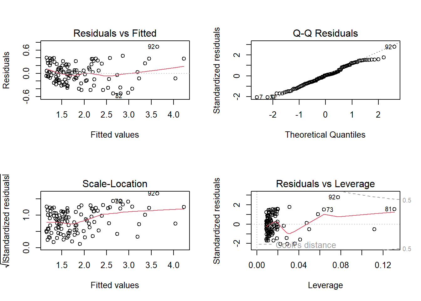
par(mfrow=c(2,2))
plot(model_bc)

library(ggplot2)
ggplot(midterm1, aes(x = mainshock, y = aftershock)) +
geom_point() +
geom_smooth(method = "lm", se = FALSE, color = "red", linetype = "dashed") +
theme_minimal(base_size = 14) +
labs(x = "Mainshock Magnitude", y = "Aftershock Magnitude",
title = "Initial Relationship Between Mainshock and Aftershock")

`geom_smooth()` using formula = 'y ~ x'

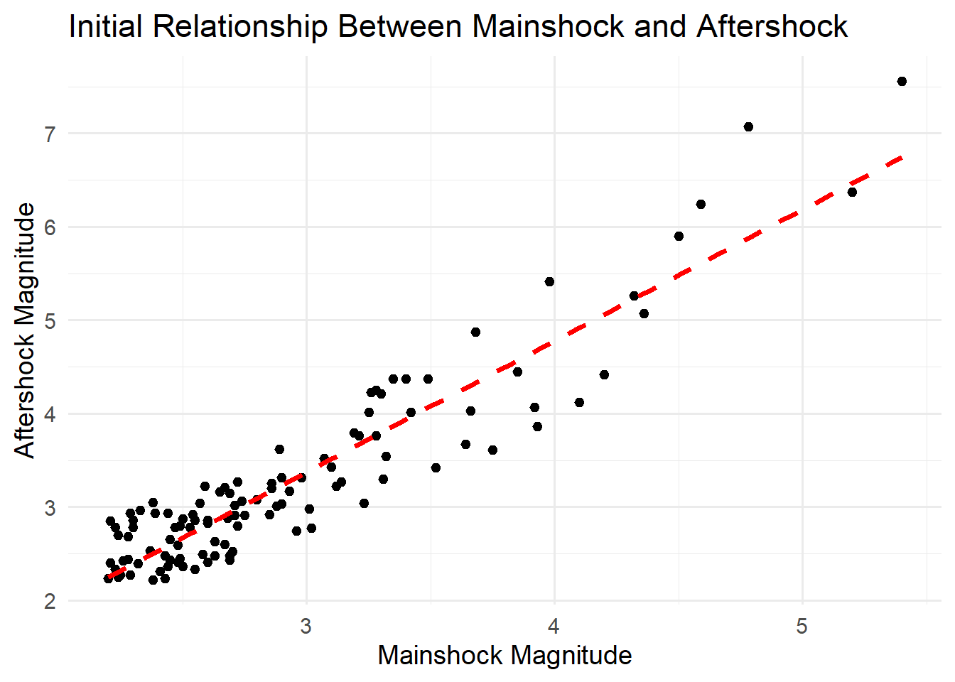
Scatterplot of Mainshock vs Aftershock Magnitudes

PART B
mainshock of magnitude 5.0 is expected to be followed by an aftershock of around 6.27 magnitude, with 95% confidence that the true mean aftershock lies between 6.01 and 6.53.

This supports the idea that as mainshock magnitude increases, the aftershock magnitude also tends to rise in a predictable, nearly linear way.

pred_bc <- predict(model_bc,
                   newdata = data.frame(x = 5),
                   interval = "confidence")
# Back-transform
yhat_conf <- (lam * pred_bc + 1)^(1/lam)
yhat_conf

       fit      lwr      upr
1 6.270939 6.012455 6.532373

PART C

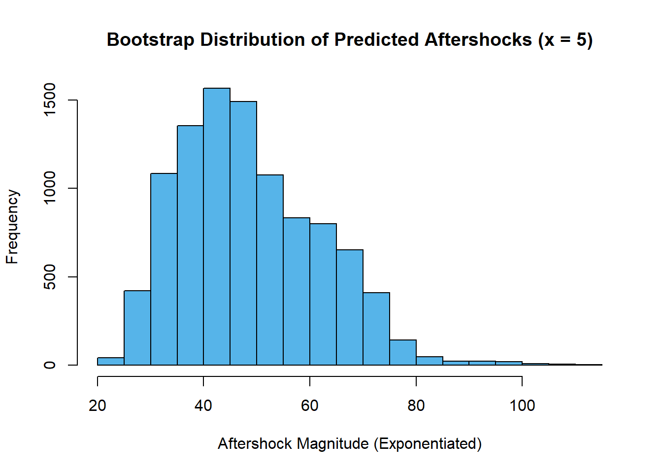
For a mainshock of magnitude 5.0, we are 95% confident that the next aftershock will fall between 5.45 and 7.07 in magnitude.

This indicates that while a 6.0 aftershock is quite plausible, magnitudes as low as 5.4 or as high as 7.0 could also reasonably occur, given the natural variability in the data.

set.seed(1254)
n <- length(x)
orig_res <- model_bc$residuals
BS.ystar <- numeric(10000)

for (i in 1:10000) {
  BS.x <- sample(x, n, replace = TRUE)
  BS.res <- sample(orig_res, n, replace = TRUE)
  BS.gyhat <- predict(model_bc, newdata = data.frame(x = BS.x))
  BS.gy <- BS.gyhat + BS.res
  BS.model <- lm(BS.gy ~ BS.x)
  BS.ystar[i] <- predict(BS.model, newdata = data.frame(BS.x = 5)) +
                 sample(orig_res, 1)
}

low.bound <- sort(BS.ystar)[250]
high.bound <- sort(BS.ystar)[9750]

# Back-transform
low.bound <- (lam * low.bound + 1)^(1/lam)
high.bound <- (lam * high.bound + 1)^(1/lam)

low.bound

[1] 5.450253

high.bound

[1] 7.073021

mean(exp(BS.ystar) > 6)

[1] 1

hist(exp(BS.ystar),
breaks = 30, col = "#56B4E9",
main = "Bootstrap Distribution of Predicted Aftershocks (x = 5)",
xlab = "Aftershock Magnitude (Exponentiated)")
abline(v = exp(c(low.bound, high.bound)), col = "red", lty = 2, lwd = 2)

Bootstrapped Prediction Interval for x = 5